1. Basic Nuclear Physics

Quick Links

• Unit 1 : Worked Problems

• Unit 1 : Additional Problems

• Unit 1 : Equations & Terms

• Unit 1 : Flash Cards

• Unit 1 : Random Quiz

• Unit 1 : Full Quiz

• From the Reading List

  • Units, nuclear scale, nomenclature and definition: Young and Freedman. Chapter 43.1

  • Nuclear sizes and cross sections, Martin Chapter 2.2

1.1. Introduction

The modern field of nuclear physics really began with the first detection of radioactivity by Becquerel, who observed that photographic plates fogged up in proximity to uranium ore. Eventually this was determined to be due to spontaneous decay of nuclei in the ore. Rutherford went on and categorized emissions of radioactive substances, working to understand the properties of alpha, beta, and gamma ray particles.

One of the major figures in nuclear physics after this was Marie Curie. She and husband Pierre were the first to isolate and characterize radium. Marie Curie’s ground breaking work led to the Nobel Prize in 1903. Her research was conducted in a time when the dangers of radiation were less well known, and Marie Curie’s lab equipment and notebooks are still highly radioactive to this day.

Quote

“I am one of those who think like Nobel, that humanity will draw more good than evil from new discoveries.” - Marie Curie

In this course we will learn about the fascinating field of nuclear physics, covering the structure of individual nuclei, predicting the properties of different radioactive decays, and both the practical applications and dangers of nuclear radiation.

1.2. Nuclear Isotopes

To begin let’s go over some fundamental nonmeclature. Isotopes are nuclei of a given element with a specific number of nucleons. They are commonly referred to by their atomic mass number, \(A\), atomic number \(Z\), and elemental symbol, \(\bf S\). For example:

• \(\bf ^{238}_{92}U~\)is an isotope of uranium with \(A=238\) nucleons (\(Z=92\) protons and \(N=146\) neutrons),
  

• \(\bf ^{56}_{26}Fe~\) is an isotope of iron with \(A=56\) nucleons (\(Z=26\) protons and \(N=30\) neutrons).
  

Since the elemental symbol is determined by the number of protons typically we ignore the bottom number to save writing it every time. For example for uranium the following five terms are all valid

(1.1)\[\begin{equation} \textnormal{U238}~=~{\bf _{92}^{238}U}~=~{\bf ^{238}U}~=~\textnormal{U-238}~=~\textnormal{Uranium-238}. \end{equation}\]

Similarly we don’t need to specify the number of neutrons, \(N\), explicitly each time as this can be determined from \(A=Z+N\). Throughout this course the short hand form of \(^{A}{\bf S}\) or \(\textnormal{S-A}\) will be used to refer to nuclei so you should familiarize yourself with it.

1.3. Radium, Radon, and the U-238 Chain

Radioactive decay of nuclei can transmute one isotope into another with the emission of some form of radiation. The most common forms of radioactive decay for nuclei are spontaneous alpha emission, or beta-decay where a neutron decays into a proton releasing an electron. As shown in the Fig. 1.1 below we can represent one nucleus decaying into another by considering where each nucleus lies on a chart of \(N\) versus \(Z\). The most common forms of decay, alpha and beta decay, have their own characteristic steps through this \(Z-N\) space.

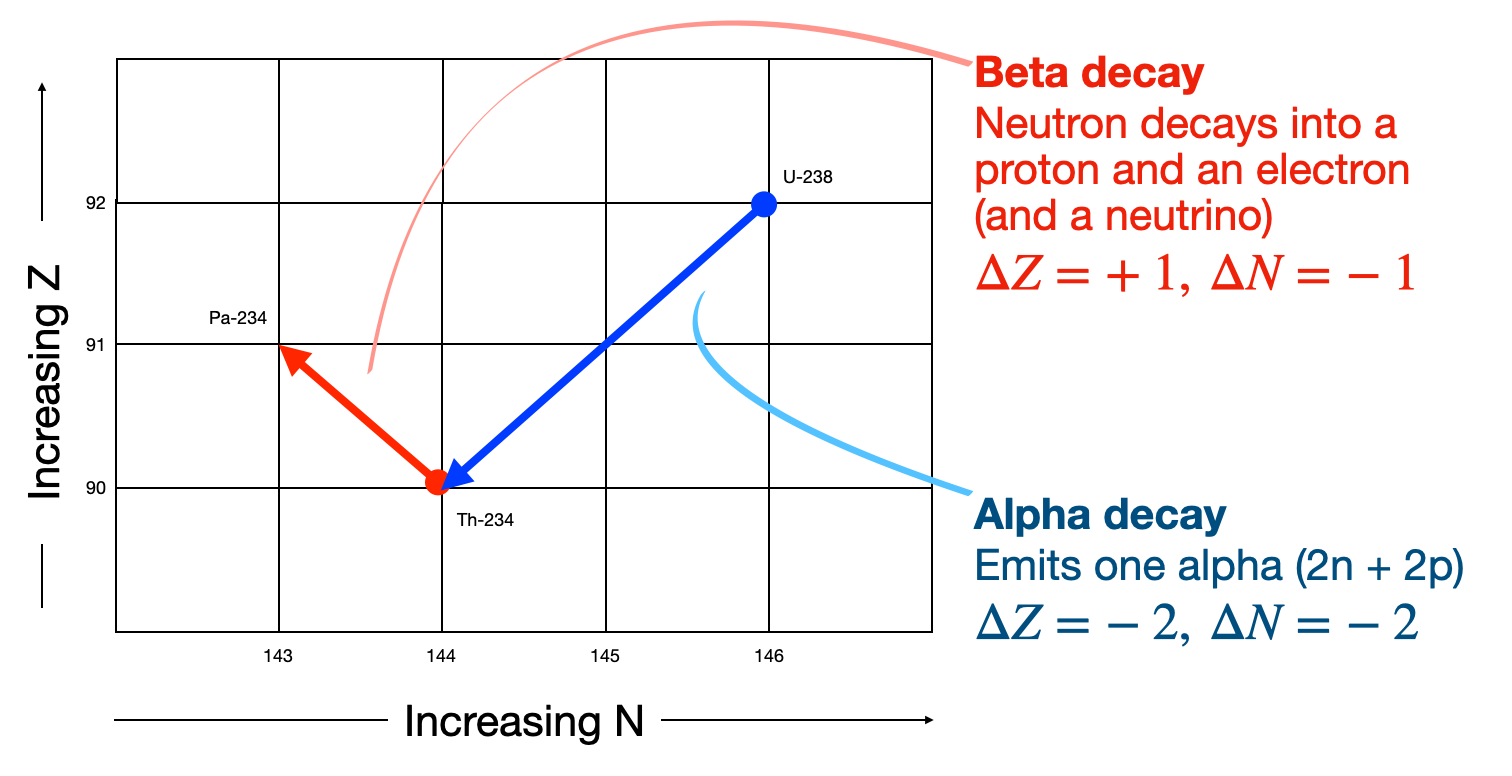
Fig. 1.1 Example how to interpret a decay chain transition diagram. Nuclei are plotted as a function of \(N\) and \(Z\). Different types of nuclear decays move around the chart in a characteristic way like chess pieces on a board.

The daughter nuclei from a radioactive decay are not necessarily always stable. When one nuclei decays into another nuclei which may at some later time also decay, these are called Decay Chains. Radium, \(^{226}{\bf Ra}\), is one radioactive isotope in a very important chain of isotopes that starts with \(^{238}{\bf U}\) and ends with \(^{206}{\bf Pb}\). As you can see in Fig. 1.2 below the decay chain can span 20 different nuclei if left long enough before finally ending at lead \((^{206}{\bf Pb})\) which is a stable end product that does not decay.

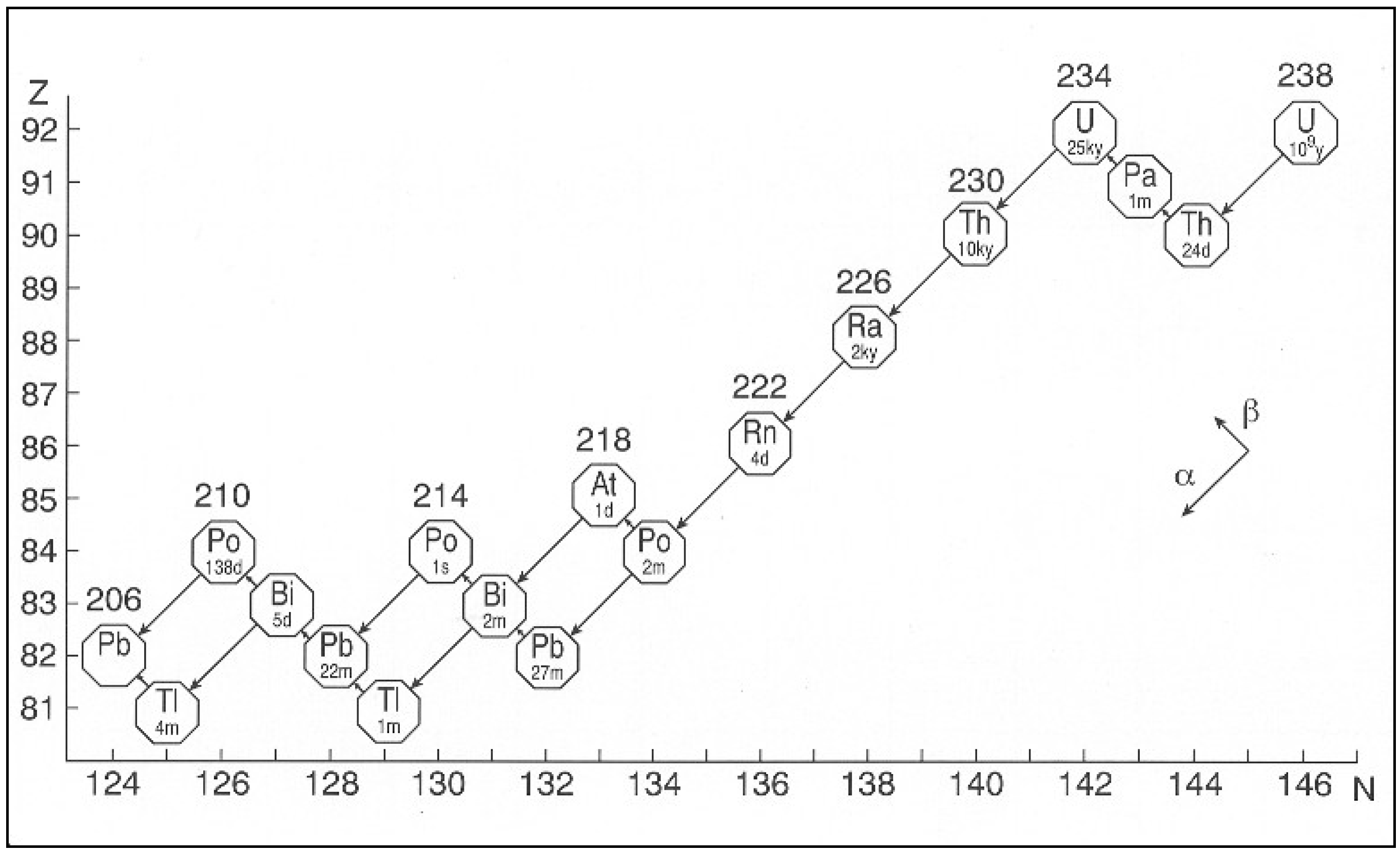
Fig. 1.2 Decay chain diagram for the U-238 chain. The approximate half-lives for each element are shown underneath them.

The decay rate of radioactive nuclei ire dependent on the isotope and as shown in Fig. 1.2 above they can vary significantly. Decay half-lives between gigayears down to seconds are observed in the \(^{238}{\bf U}\) chain. Radon occurs in the middle of the \(^{238}\textnormal{U}\) chain and has serious health implications. It is an alpha emitter so when outside our bodies it can’t cause much harm. As shown in Fig. 1.3 since it is commonly a gas, it can enter the lungs and cause damage to cells. With a half life of 3 days it is a particular problem in underground locations as it can manifest from rocks and hang around in the air for several days before it is inhaled. Radon is actually the major source of natural background radiation that can be harmful to us.

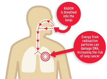
Fig. 1.3 Radon gas typically emits alpha particles. Outside the body these cannot do much damage as they are not penetrating. However when inhaled alpha particles can cause major damage to cells in the lungs.

1.4. Radiation Hazards

Radiation in general is quantified in various units. For experimental physics the source activity in Becquerels is often considered. For health the most important is the Gray and Sievert.

• A Becquerel is a measure of source activity. It corresponds to the number of radioactive decays per second (so is correlated with the number of high energy particles leaving the source).

• A Gray is \(1~\textnormal{J/kg}\) of deposited energy. This depends on the source and it’s activity, but also the stand-off distance to the source itself as radiation intensity falls off based on the inverse square law.

• The Sievert is a Gray multiplied by a dimensionless quantity \(Q\) with value depending in the type of particle. \(Q\) represents the different levels of damage that different particles can do to human cells. An alpha has a high \(Q\) Value because it does more damage to tissue than say electrons of the same energy.

Whilst a measurement in Becquerel’s tells us how active a source is, the most important measure throughout applied nuclear physics is the Sievert. A dose of one Sievert is lethal. The allowed dose for workers in the UK is 20 millisieverts per year. This is governed by UK IRR2017 regulations.

Here is a summary of various units used throughout the nuclear physics field:

Tables	Source Activity	Absorbed Dose	Effective Dose	Intensity
Old unit	Curie	Rad	Rem	Roentgen
SI unit	Becquerel	Gray	Sievert	…

Note

You’ll notice that there is no current SI unit for intensity anymore. This is because measurement of intensity of a source at some standoff distance is somewhat arbitrary. Roentgen’s are sometimes still used for this but commonly the effective dose at some distance is the quantity of interest. In radiation detector development commonly “\(y\) Becquerels at distance \(x\)” or “\(y\) mCuries at distance \(x\)” is used to define a reference source intensity at a given position.

1.5. Basic Properties of Nuclei

Now our challenge over the course of this module is to understand the structure of individual nuclei and the impact this has on observables such as different types of radioactive decays.

To do this we need to review what properties of nuclei and their behavior we can directly observe. We’ll start with some basic nomenclature and properties of Nuclei. As we mentioned before nuclei can be described in terms of:

• Number of protons (atomic number): \(Z\)

• Number of neutrons : \(N\)

• Number of nucleons (atomic weight) : \(A=Z+N\)

Nuclei can also be grouped according to their \(Z\), \(N\), and \(A\) values:

• Nuclides with the same \(Z\) are Isotopes

• Nuclides with the same \(A\) are Isobars

• Nuclides with the same \(N\) are Isotones

The known elements cover essentially everything from Hydrogen, H-1 to Oganesson-294. {numref}chart-of-nuclideslarge` is a chart showing different known nuclei. Around 3000 different nuclei have so far been confirmed, each specified by the proton number \((Z)\) and neutron number \((N)\). This nuclide plot is one of the most important plots in nuclear physics.

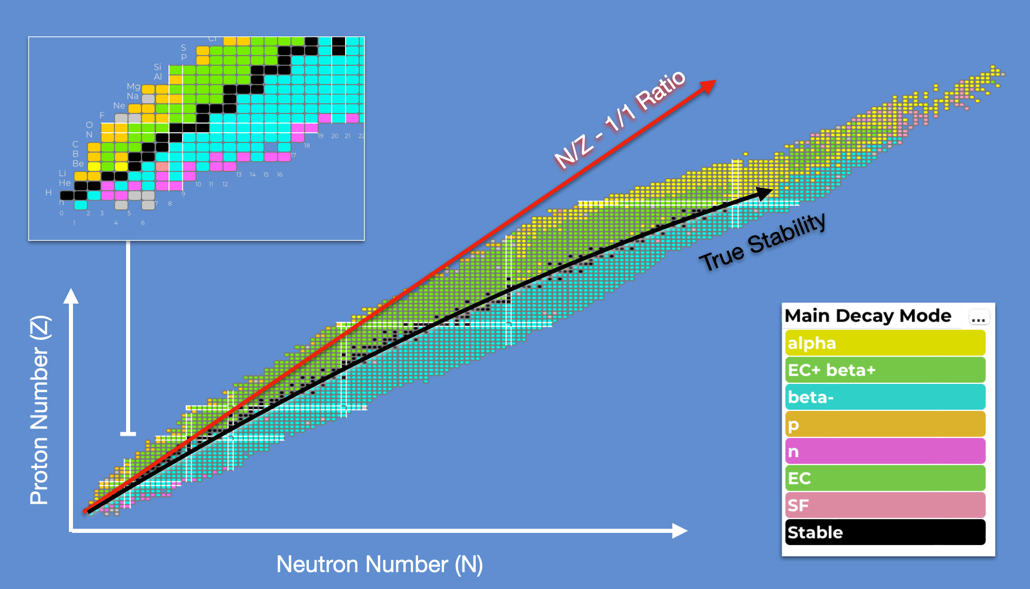
Fig. 1.4 Chart of all known nuclides. All observed nuclei are given a square based on their \(N\) and \(Z\) value. As we move away from the black line in both directions the nuclei become more and more unstable. At higher \(Z\) values we need more neutrons to counteract electrostatic repulsion and make the nucleus stable.

The most stable elements run along what is called the “Line of Stability” when plotted as a function of \(Z\) and \(A\). Nuclei that deviate from this line decay rapidly to more stable nuclei, converting excess neutrons to protons if below the line (beta+ decay or Electron Capture) or converting excess protons to neutrons if above the line (beta- decay). The light elements have a strong tendency for \(N\)=\(Z\) whilst for heavier elements the relationship follows something closer to \(N=1.5\times Z\).

Note

Remember : Unstable nuclei want to head towards more stable states - towards the line of stability.

The international atomic energy agency (IAEA) has gone to great lengths to catalogue information on nuclear physics and radioactive decays. They provide a full library of the properties of each known nuclei in this plot. A link to the IAEA’s interactive nuclei viewer can be found here.

1.6. Nuclear Decay

As we mentioned earlier, nuclei sometimes decay in chains until a more stable state is reached. The N and Z values for these stable states usually lie somewhere along the Line of Stability. Whilst we’ve discussed the dominant decays in the U-238 chain, there are actually six types of nuclear decay we need to remember.

1. Alpha Decay - Spontaneous emission of an \(\alpha\) particle, \(\Delta Z=-2, \Delta N=-2\)

2. Beta Decay - Spontaneous decay of a neutron into a proton and an electron, \(\Delta Z=+1, \Delta N=-1\)

3. Neutron Emission - Spontaneous ejection of a neutron from the nucleus, \(\Delta Z=0, \Delta N=-1\)

4. Proton Emission - Spontaneous ejection of a proton from the nucleus, \(\Delta Z=-1, \Delta N=0\)

5. Positron Emission - A proton emits a positron and turns into a neutron , \(\Delta Z=-1, \Delta N=+1\)

6. Electron Capture - A proton captures an orbiting electron, turning into a neutron and emitting a neutrino. \(\Delta Z=-1, \Delta N=0\)

The possible steps for these on our chess board of decays are shown in.

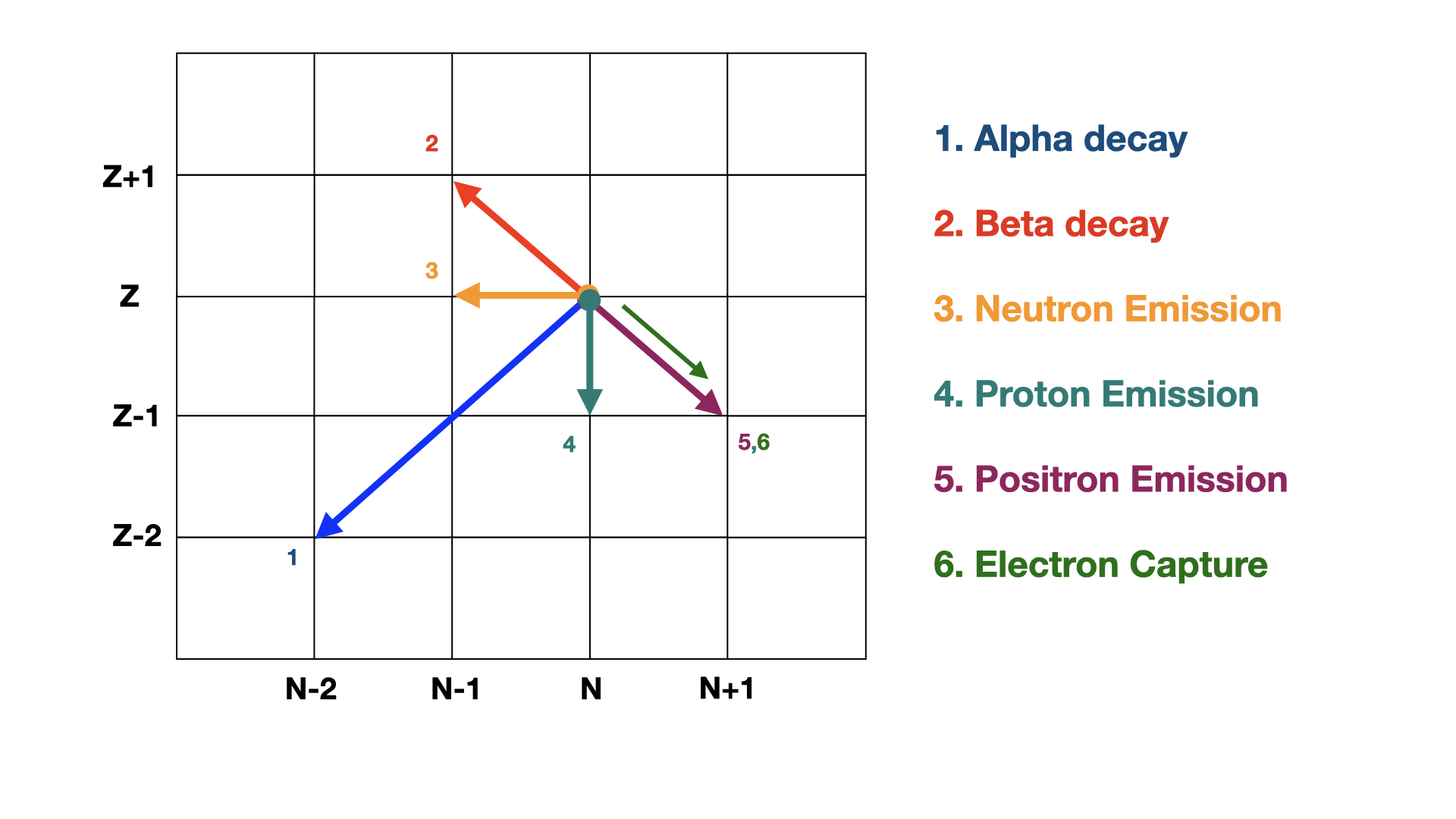
Fig. 1.5 Possible decay steps in a chart of nuclides. Different decay channels correspond to different steps through the grid. The most common decays are still Alpha and Beta decay.

1.7. Mass Calculations

Differences in mass between different nuclei plays a major role in their relative stabilities. Obviously every nucleus carries mass, but this turns out to be more complicated than you might think and we cannot simply add up the masses of the nucleons inside to get the total of the bound state.

Once collections of nucleons are together inside a nucleus they generally want to stay together (at least for the most stable nuclei!). It takes additional energy to pull a nucleus apart - this is called the Binding Energy, and it is why we cannot simply add the mass of the nucleons together when determining the nuclear mass.

It is also important to understand if we are considering Nuclear Mass or Atomic Mass. A nucleus is the part of an atom that is made only of protons and neutrons (nucleons). If electrons are included, then we have an atom (neutral or ionized depending on the number of electrons). The mass of an atom is dominated by the nucleons so in many cases in nuclear physics it is a reasonable assumption to assume the atomic mass is the same as the nuclear mass. However, this is not always true, for instance in some beta decay calculations, we need to account for this as we will see later. Remember that in nuclear physics we tend to deal with energies (masses) in the MeV range. Whereas for electrons in orbitals (Atomic Physics) we consider eV and keV scales.

To make our lives easier when carrying around a lot of \(\textnormal{MeV}\) terms in nuclear physics it is helpful to define a standard mass close to the nucleon mass. This is the Unified Mass Constant (\(u\)). Nuclear masses are typically expressed in terms of unified mass constant (\(u\)). The mass of a C-12 atom is defined to be exactly \(12u,\) so that

(1.16)\[\begin{equation} u = 1.66056\times 10^{-27}~\textnormal{kg} = 931.5 \textnormal{MeV/c}^2. \end{equation}\]

This results in the proton, neutron, and electron masses being defined as:

• \(m_p\) = \(1.672\times 10^{-27}~\textnormal{kg}\) = \(1.007276~u\) = \(938.28~\textnormal{MeV/c}^2\)

• \(m_n\) = \(1.675\times 10^{-27}~\textnormal{kg}\) = \(1.008665~u\) = \(939.57~\textnormal{MeV/c}^2\)

• \(m_e\) = \(9.109\times 10^{-31}~\textnormal{kg}\) = \(0.000549~u\) = \(0.511~\textnormal{MeV/c}^2\)

  
  

You’ll see already from these definitions that the mass of a free proton or a neutron is more than \(u\) itself by between 0.7-0.8%. This is quite important as we defined \(u\) based on the mass of C-12 divided by it’s number of nucleons. This means a carbon atom is also approximately 0.8% lighter than the sum of its constituents. We find that this is true for all nuclei. The mass of a given nucleus is always less than the sum of the masses of the individual nucleons inside. This is because the forces that hold nuclei together contribute additional negative energy,

(1.3)\[\begin{equation} M(A,Z) < Zm_{p} + Nm_{n}. \end{equation}\]

This nuclear mass deficit can be calculated as the difference between the nuclear mass, and the sum of individual nucleons.

(1.4)\[\begin{equation} \Delta M(A,Z) = M(A,Z) - (ZM_{p} + NM_{n}). \end{equation}\]

Note

Note that in the equation above we haven’t included the electron masses. This contributes several percent for low mass nuclei so in some cases can’t be neglected. The important point to determine if electron masses should be included is in whether the mass of just the nucleus \(M(A,Z)\) is given, or the mass of the neutral atom is given \(M_{atom}\).

The deficit shown in Eq. (1.4) is related to the binding energy, \(B\) of nuclei, corresponding to the total energy required to split the nucleus apart into free nucleons

(1.5)\[\begin{equation} -\Delta M(A,Z) = B \end{equation}\]

Typically the binding energy is referred to as a positive value, but when considering its role in calculating the overall mass of the nucleus the change in mass is actually negative as shown in Eq. (1.5). As we discussed in the last lecture, stable nuclei have the highest binding energies - it takes more to pull them apart.

For a worked example related to binding energies see : Example 1.1 : Carbon Mass Calculation

Since the neutrons and protons have different masses and properties, we expect that the binding energy for neutrons or protons to be very slightly different. These individual binding energies are commonly referred to as Separation energies. For example, the neutron separation energy for a Carbon-12 atom is calculated by taking the difference in binding energies between Carbon-12, and Carbon-11 (one less neutron). Similarly the proton separation energy for C-12 is calculated from the difference between C-12 and N-12.

Note

Setting \( c = 1 \) in Nuclear Physics

In nuclear physics, it is common to set the speed of light (\( c \)) equal to 1. This simplifies calculations by expressing mass, energy, and momentum in the same units, typically mega-electronvolts (\( \text{MeV} \)). For example, rather than writing mass as \( \text{MeV}/c^2 \), it is simply expressed in \( \text{MeV} \).

Why This Works If we consistently work in natural units, where \( c = 1 \) and \( \hbar = 1 \), it can make equations easier to manipulate without repeatedly including factors of \( c \) or \( \hbar \).

Example The rest energy of a proton is \( m_p = 938 \, \text{MeV}/ c^2 \). Setting \( c = 1 \), we directly express the proton’s mass as \( m_p = 938 \, \text{MeV} \), simplifying equations like:

\[E^2 = p^2 + m^2 \quad \text{(instead of $ E^2 = (pc)^2 + (mc^2)^2 $)}.\]

This convention streamlines calculations without sacrificing accuracy we just have to remember to use MeV/c\(^{2}\) for mass and MeV/\(c\) for momentum consistently.

Below in Fig. 1.6 is the second most important plot in nuclear physics. It is a plot of the Average Binding Energy per total number of nucleons (\(A=Z+N\)) for all nuclei.

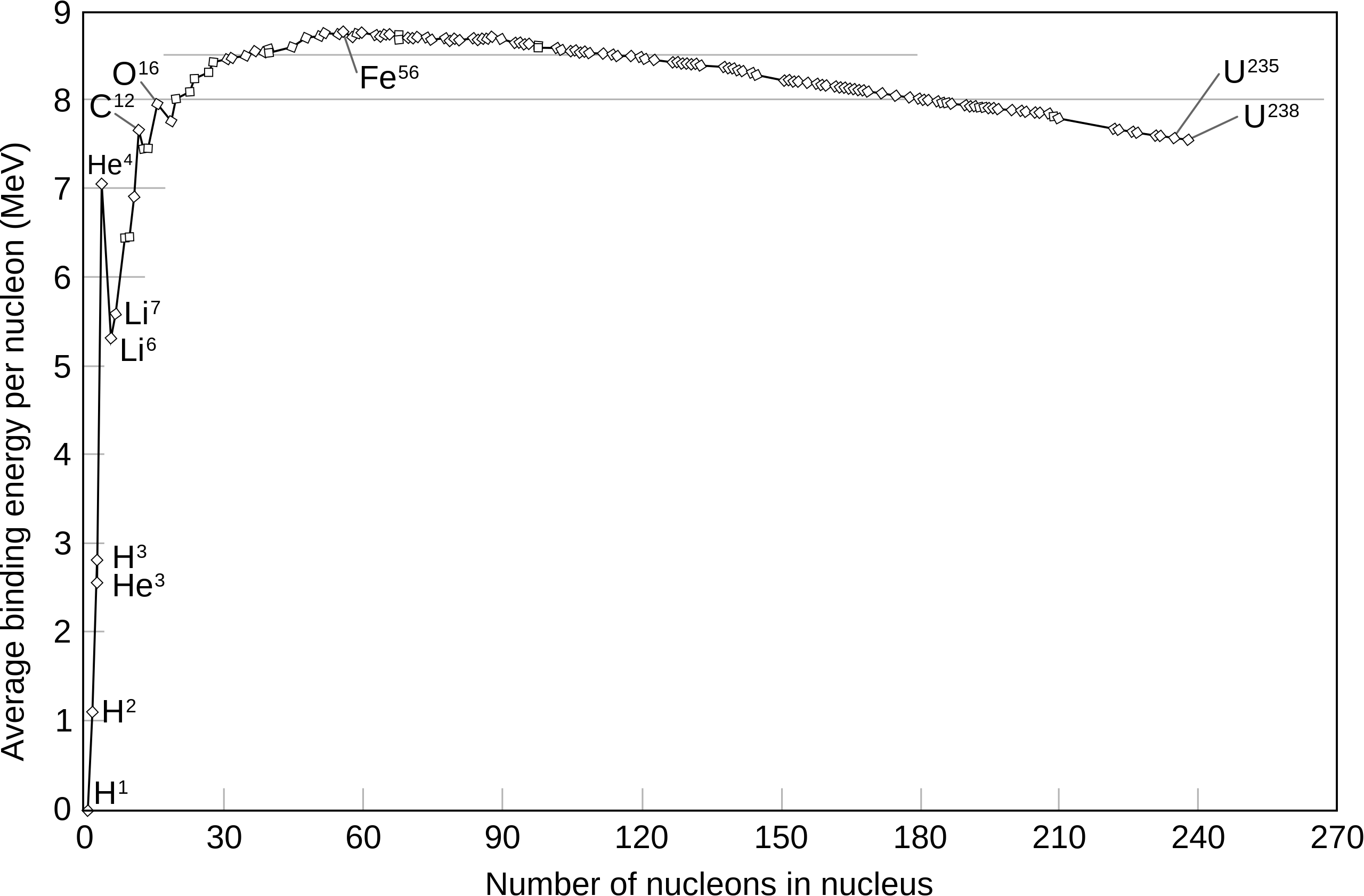
Fig. 1.6 Plot of average binding energy per nucleon versus number of nucleons in the nucleus. A peak is observed at Fe-56, above which the binding energy reduces as larger nuclei become less tightly bound.

There are some very important features here already that we should consider:

1. For heavy nuclei the binding energy is stable at around \(8~\textnormal{MeV/nucleon}\).

2. The maximum binding energy is at \(A=56\) which is Iron. \(\textnormal{Fe-56}\) is one of the most stable well-bound nuclei.

3. Local peaks are visible when \(A=4N\), e.g. \(\textnormal{He-4}\). These features play important roles in how we build nuclear models as we will see later in the course.

You may have seen this plot already in second year nuclear physics, and may even understand the implications of these features, but in this course we are going to delve a bit deeper into actually where these features and look at how we construct models that can accurately describe this plot, and explain each of the decay phenomena we have discussed in this lecture in more detail.

1.8. Probing the Nucleus

Nuclei as opposed to atoms, have a net charge, from the sum of the proton charges. Neutrons can be considered essentially neutral, as the name suggests. However, in fact we know both neutrons and protons have an internal structure. Neutrons are composed of 3 quarks, (up, down, down for neutrons) that all have charge. The sum of the charges is zero but the structure does mean that charge-like phenomena exist for neutrons arising from their internal charge distribution. For example the neutron has a non-zero magnetic moment.

The fact that nucleons consist of quarks is actually the reason nuclei form in the first place. The nuclear force that binds nuclei together is in itself not a fundamental force. Instead the nuclear force is mediated by virtual pions (particle made of a quark and anti-quark) being exchanged between nucleons as a result of strong interactions. The nuclear force can therefore be thought of almost as a leakage of the strong force which reaches a very small range outside of each nucleon.

Of course nuclei also have finite size, but it’s impressively small when compared to the size of the electron orbitals in an atom, and the scale of the nuclei itself is typically only one to two orders of magnitude greater than nucleons themselves. A comparison of relative scale differences in the relative sizes for some nuclei shown in Fig. 1.7.

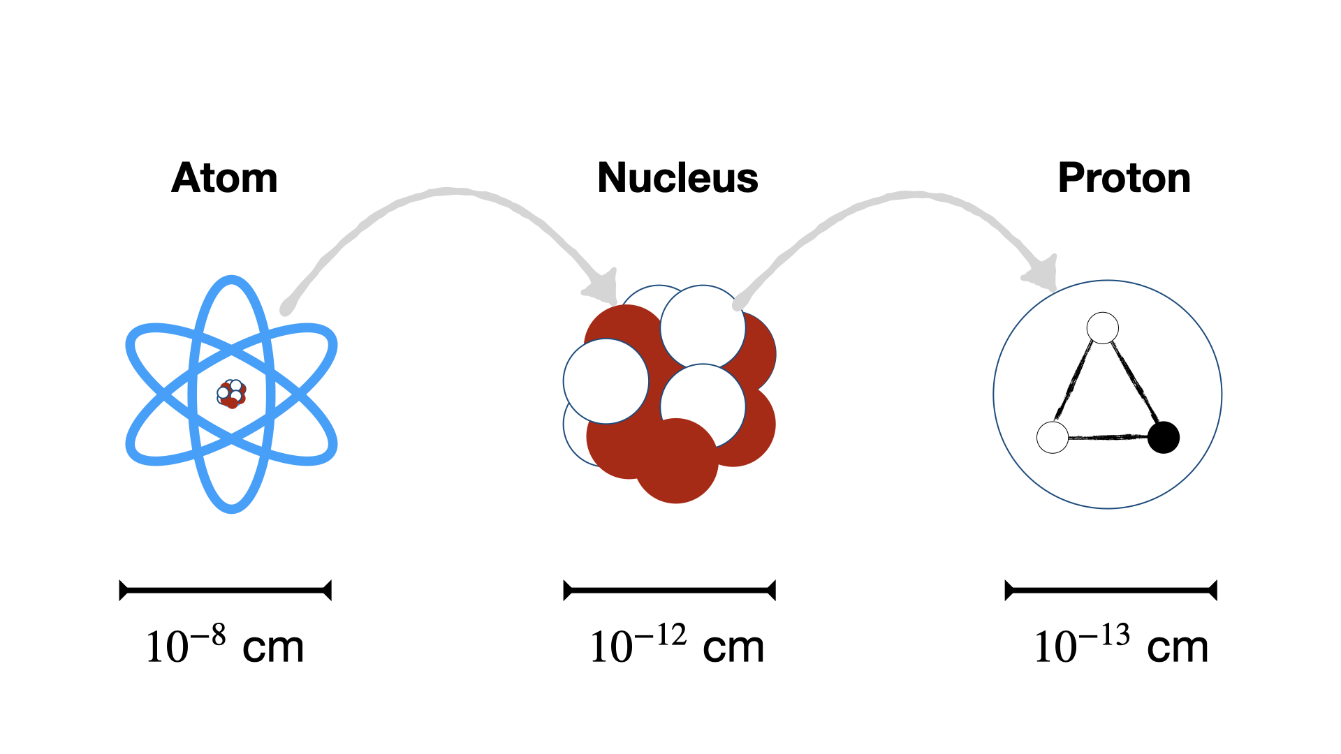
Fig. 1.7 Atomic versus Nuclear versus Proton size comparisons

Example scales of Aluminium

• Atomic Radius of Aluminium = \(1.3 \times 10^{-10}~\textnormal{m}\)

• Nuclear Radius of Aluminium = \(3.6 \times 10^{-15}~\textnormal{m}\)

Given that Nuclei have mass and charge then there is obviously going to be a density of mass and charge in nuclei, with some distribution. We’ll consider this in more detail later. For now we can ask what is the average mass and charge density of the nuclear material. To estimate this simply assume that nuclei are made of nucleons (protons and neutrons) that are something like Hard Spheres of radius \(r_{0}\). The density is then estimated assuming each nucleon is packed together but doesn’t overlap. This allows the mass density to be approximately the same as a single nucleon density as

(1.6)\[\begin{equation} \rho_{m} = \frac{M}{V} = \frac{3m_{n}}{4\pi r^{3}_{0}} \end{equation}\]

where \(m_{n}\) is mass of neutron. For charge a similar approach can be taken but we have to include the fact that neutrons have no charge, and it is only every proton that contributes a single charge \(e\) to the total charge \(Q\) of the nucleus.

(1.7)\[\begin{split}\begin{equation} \rho_{c} = \frac{Q}{V} = \frac{3Ze}{4\pi r^{3}_{0} A}\\ \end{equation}\end{split}\]

For a worked example related to nuclear size see : Example 1.2 : Nucleon Momentum Estimate

1.9. Measuring Nuclear Size

To get a better idea of the actual size, charge, and matter distribution, physicists use Scattering Experiments. The typical approach is to fire beams of particles at a fixed target and see what has happened to the particles on the other side.

Typical experiments are : (i) electron scattering, (ii) alpha particle scattering, (iii) proton scattering, and (iv) neutron scattering and absorption.

For best results the de Broglie Wavelength of the probing nuclei must be a smaller than the nucleus, some typical beam energy values for nuclear probe experiments:

• alphas \(>\) 2 MeV

• protons \(>\) 8 MeV

• electrons \(>\) 120MeV

Note

Remember the de Broglie Wavelength is the wavelength of the probing beam of particles which can be calculated from the momentum via \(\lambda = h/p\).

A vital concept in such experiments is the notion of Interaction Cross Sections. The Cross Section \(\sigma\), quantifies the probability of a collision (or reaction) occurring between a beam particle and a target particle. It is based on the probability an interaction occurs using the notion of a Cross Sectional Area for the nucleus. It can be defined as an area around the centre of one of the particles within which the centre of second must fall if they are to collide as illustrated in Fig. 8.

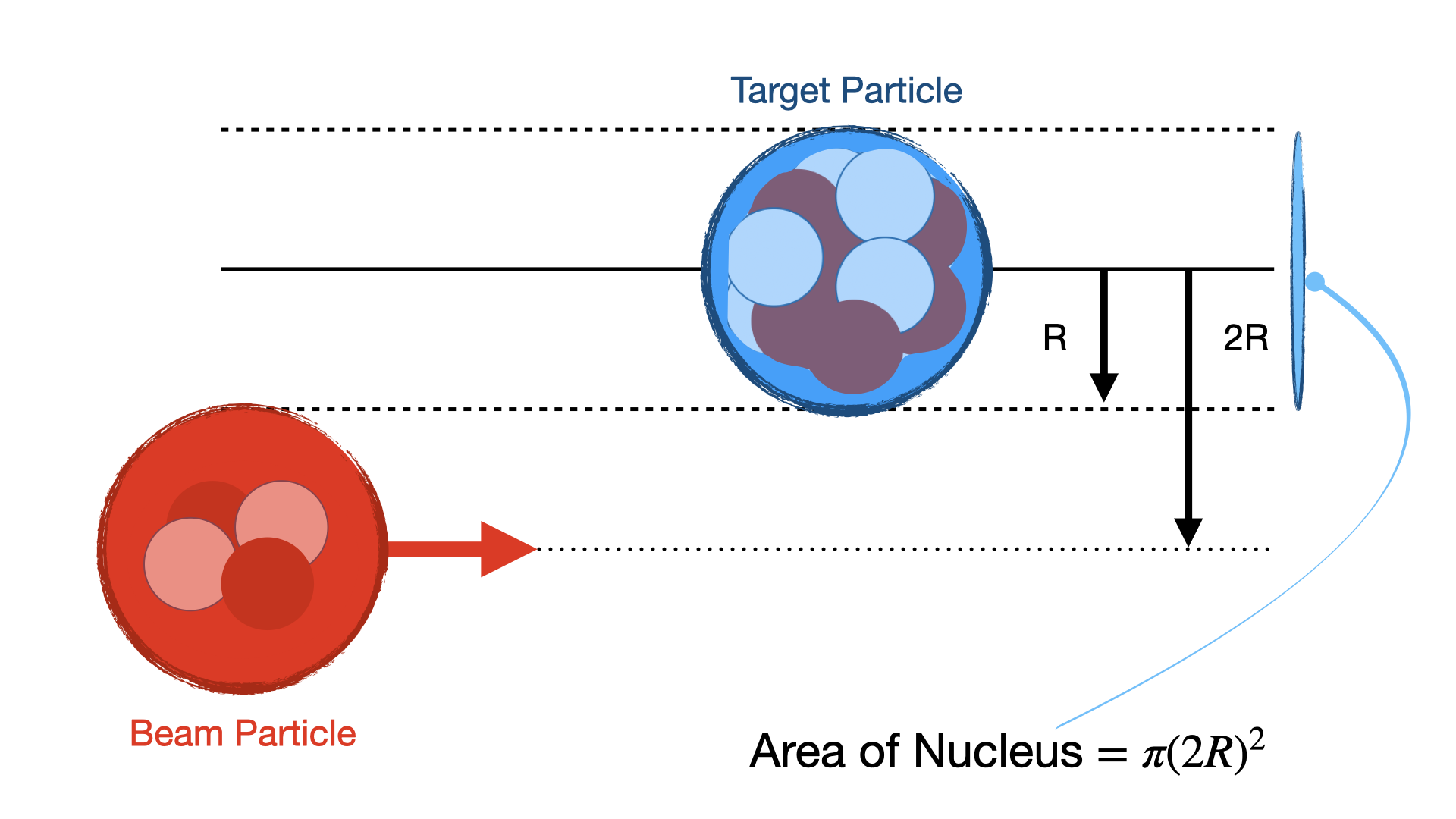
Fig. 1.8 Cross-section calculation based on assuming interacting bodies are hard spheres. If the center of the particle on the left is within \(2R\) of the the one on the right then the particles will interact with one another.

Normally we can assume the particles are simple Hard Spheres such that if they all have radius R then the cross-sectional area is just,

(1.8)\[\begin{equation} \sigma = \pi (2R)^{2} \end{equation}\]

Due to the small sizes of nuclei, \(\sigma\), is often expressed in units of Fermi squared \((10^{-30}m^{2})\) or barns \((10^{-28}m^{2}\)) or even pico-barns\(~(10^{-40}m^{2})\). In reality, as we will see, nuclei are not hard-edged and so cross-sections cannot be defined so geometrically, but it is a reasonable approximation for now.

If we consider a material (a “Target”) with \(n\) particles per unit volume, then we can use the total cross-section, \(\sigma\), to find the Mean Free Path for an interaction by a given particle fired at that material. For a Thin Target (or Foil) this is given by

(1.9)\[\begin{equation} \lambda = \frac{1}{n\sigma}. \end{equation}\]

The mean free path or cross-section can be used to determine the reduction in beam particles for a given target. Consider we have a beam of \(N_0 ~\textnormal{particles/s}\) impinging on a target so that a flux \(N\) emerges.

For thick targets of thickness \(x\) then

(1.10)\[\begin{equation} N = N_0 e^{-x/\lambda} \end{equation}\]

and the number of collisions in distance x is

(1.11)\[\begin{equation} C=N_0-N=N_0(1-e^{-x/\lambda}). \end{equation}\]

For thin targets (\(x << \lambda\)) instead the exponential term in the can be reduced to

(1.12)\[\begin{equation} N=N_0\left(1+\frac{x}{\lambda}\right) \end{equation}\]

meaning the number of collisions becomes

(1.13)\[\begin{equation} C=\frac{xN_0}{\lambda} = N_{0}n\sigma x. \end{equation}\]

We can see from Eq. (1.10) that given accurate prior knowledge of our starting beam flux and the thickness of our target, we can determine the cross-section of the total particles inside simply by measuring the change in intensity of our beam.

For a worked example related to cross-section calculations see Example 1.3 : Shielding Cross-section Estimate

1.10. Partial and Differential Cross Sections

So far the Cross Section we have considered has really been the Total Cross Section, \(\sigma_{T}\), referring to the sum of all possible interactions involving the beam and target particles. In practice, there may be different types of interaction, or Interaction Channels, that happen each with their own seperate probability. The sum of all the cross-sections for each possible channel gives the total cross-section for the target. We introduce the term Partial Cross Section to distinguish these from the total cross-section, for instance \(\sigma_{e}\).

In the previous sums we have also not said anything about where a given scattered particle goes, i.e. the angle through which it is scattered. It could be that all scattering angles are equally likely. This would be Isotropic Scattering. In practice however some angles end up being more likely than others due to various kinematic constraints depending on the interaction. To account for this we use the Differential Cross-Section \( \frac{d\sigma}{d\Omega} \)

Consider a finite element of solid angle \(\Delta \Omega\) at angle \(\theta\) as shown in Fig. 1.9. There is a part of \(\sigma_e\) called \(\Delta \sigma_{e}\) which corresponds to a probability of scattering into that cone. The Differential Cross Section for elastic scattering at angle \(\theta\) is thus

(1.14)\[\begin{equation} \frac{d\sigma_{e}}{d\Omega} = (lim \Delta\Omega \rightarrow 0) \frac{\Delta \sigma_{e}}{\Delta \Omega} \end{equation}\]

If we integrate \(d\sigma/d\Omega\) over all possible scattering angles then we get back to the total cross section for that particular channel.

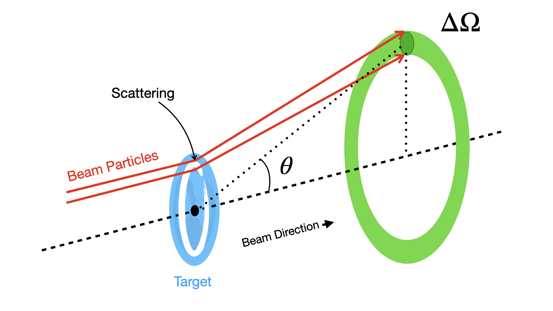
Fig. 1.9 Scattering angle cone used to define \(\Delta \Omega\) in beam scattering experiments.

Here we have considered a differential cross-section in terms of a solid angle, but in practice this can be given in terms of any kinematic variables derived from the interaction. For example the differential cross-section for electron scattering calculated in terms of the beam energy may be expressed as \(d\sigma/dE\), and a double differential cross-section in terms of beam energy and scattering angle may be expressed as \(d^{2}\sigma/(dEd\theta)\).

Addition Notation Clarification (18/02/2024) Below is an additional example of different notations used for reaction cross-sections when scattering a beam of particles, \(a\), into a target \(X\), resulting in a secondary observed beam of scattered particles, \(b\), and the production of a new radio-isotope \(Y\).

Cross Sections	Symbol	Technique	Possible Application
Total	σₜ	Attenuation of beam	Shielding
Reaction	σ	Integrate over all angles and all energies of b	Production of radioisotope Y in a nuclear reaction
Differential (Angular)	dσ/dΩ	Observe b at (θ, φ) but integrate over all energies	Formation of beam of b particles in a certain direction (or recoil of Y in a certain direction)
Differential (Energy)	dσ/dE	Don’t observe b, but observe excitation of Y by subsequent γ emission	Study of decay of excited states of Y
Doubly differential	d²σ/dEₓ dΩ	Observe b at (θ, φ) at a specific energy	Information on excited states of Y by angular distribution of b

1.11. Rutherford and Mott Scattering

The first nuclear scattering experiments, famously started by Rutherford, were performed using alpha particles. These experiments used a collimated polonium sample to create a beam of alpha particles which could be directed at a thin gold foil. A fluorescent screen was used to determine the scattering angle of the particles after the interaction. The cross-section measured in these interactions can then be used to determine the nuclear radius. Below is a sketch of Rutherfords original experiment using a gold thin foil as a target.

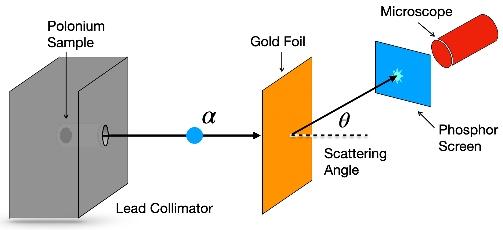
Fig. 1.10 Hyperbolic Trajectory of scattering in Rutherford scattering assuming charged deflection of the beam particles.

Two important conclusions were drawn from the early scattering experiments:

• Nuclear have very small size, about \(10^{-14}~\textnormal{m}\)

• Nuclear Radii, \(R\), are seen to increase with the total number of nucleons, \(A\), such that \(R\approx r_{0} A^{1/3}\), where \(r_{0}\) is the nucleon radius. This suggests that nucleons are Incompressible.

Rutherford and others went further after these ground breaking experiments, to deduce an equation for the angle by which alpha particles scatter, known as the Differential Cross Section for Rutherford Scattering based on assuming that alphas follow a hyperbolic trajectory as they scatter of a static point-like charge target.

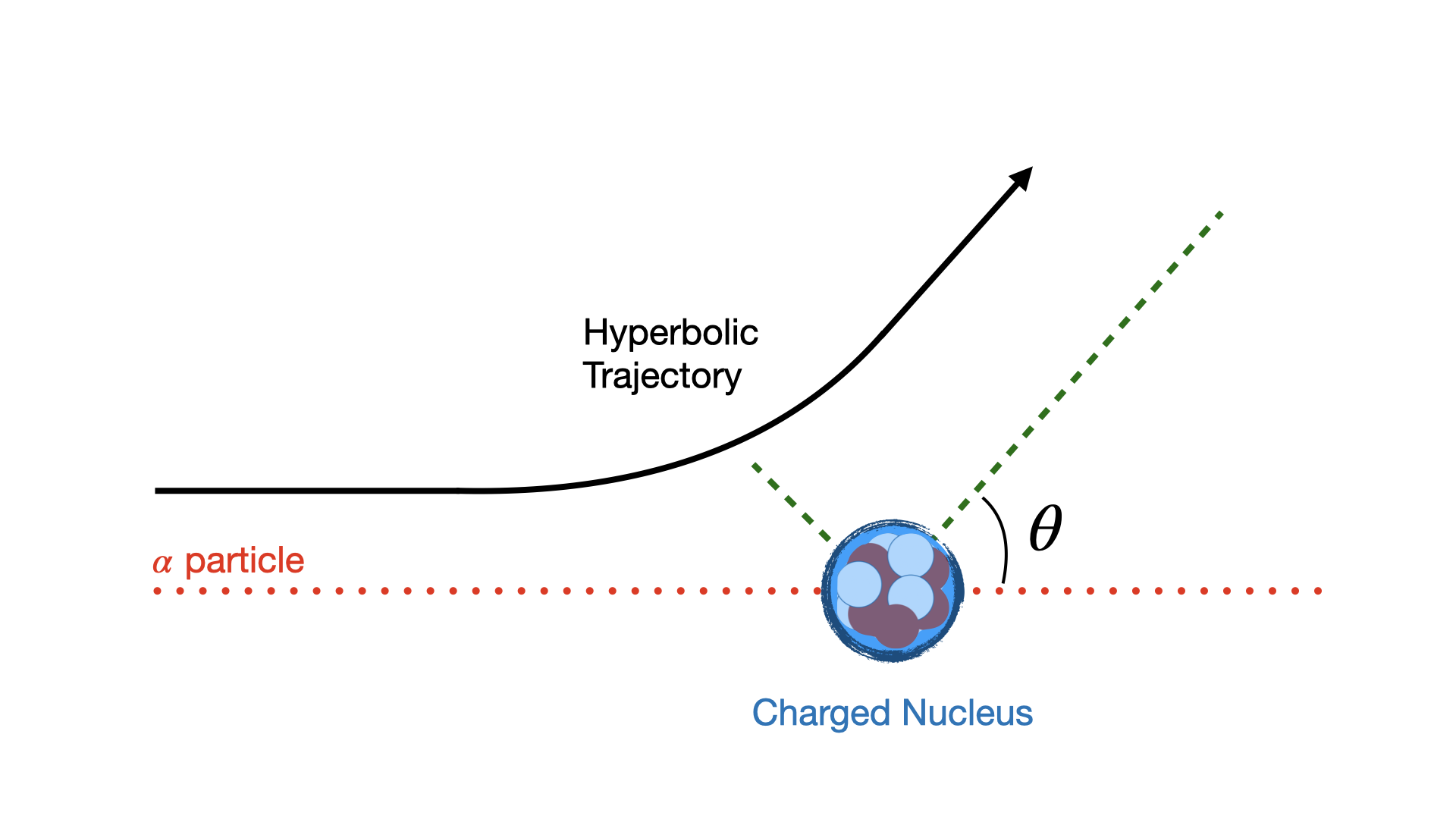
Fig. 1.11 Hyperbolic Trajectory of scattering in Rutherford scattering assuming charged deflection of the beam particles.

(1.15)\[\begin{split}\begin{equation} \frac{d\sigma}{d\Omega_{R}} = \frac{z^{2}Z^{2}\alpha^{2}\hbar^{2}c^{2}}{4E^{2}} \frac{1}{sin^{4}(\theta/2)} \\ \end{equation}\end{split}\]

• \(z\) is the charge of the projectile.

• \(Z\) is the charge of the scatterer.

• \(E\) is kinetic energy of the particle

• \(\theta\) is the scattering angle

• \(\alpha\) is the fine structure constant

Note

The fine structure constant defines the strength of electromagnetic interactions.

(1.16)\[\begin{equation} \alpha = \frac{e^{2}}{\hbar c 4\pi \epsilon_0} \end{equation}\]

{numref}`rutherfordform predicts a form the cross section vs scattering as shown opposite.

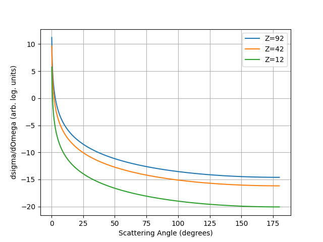
Fig. 1.12 Rutherford Cross-section Form for three different nuclei.

For a worked example related to rutherford scattering closest approach see Example 1.4 : Closest Approach Estimate.

Unfortunately the Rutherford prediction has been found to give a poor fit to real data. The main reason being the assumption that alphas are point-like objects. An improvement, introduced by Mott, is to use electrons, that are indeed point-like and can also better probe the nucleus, if of sufficient energy. This requires taking account of the relativistic effects of high energy electrons, their Magnetic Moment and also the resulting Nuclear Recoil.

The result is a modification to the equation above, thus:

(1.17)\[\begin{equation} \frac{d\sigma}{d\Omega_{M}} = \frac{d\sigma}{d\Omega_{R}} \times [1-\beta^{2} sin^{2} (\theta/2)] \end{equation}\]

where \(\beta\) encompasses these corrections for relativistic electrons.

Hofstadter set up electron scattering experiments on nuclei to investigate the Mott scattering prediction, illustrated in Fig. 1.13 below. These experiments used electrons of 500 MeV to probe down to length scales of \(2.5~\textnormal{fm}\).

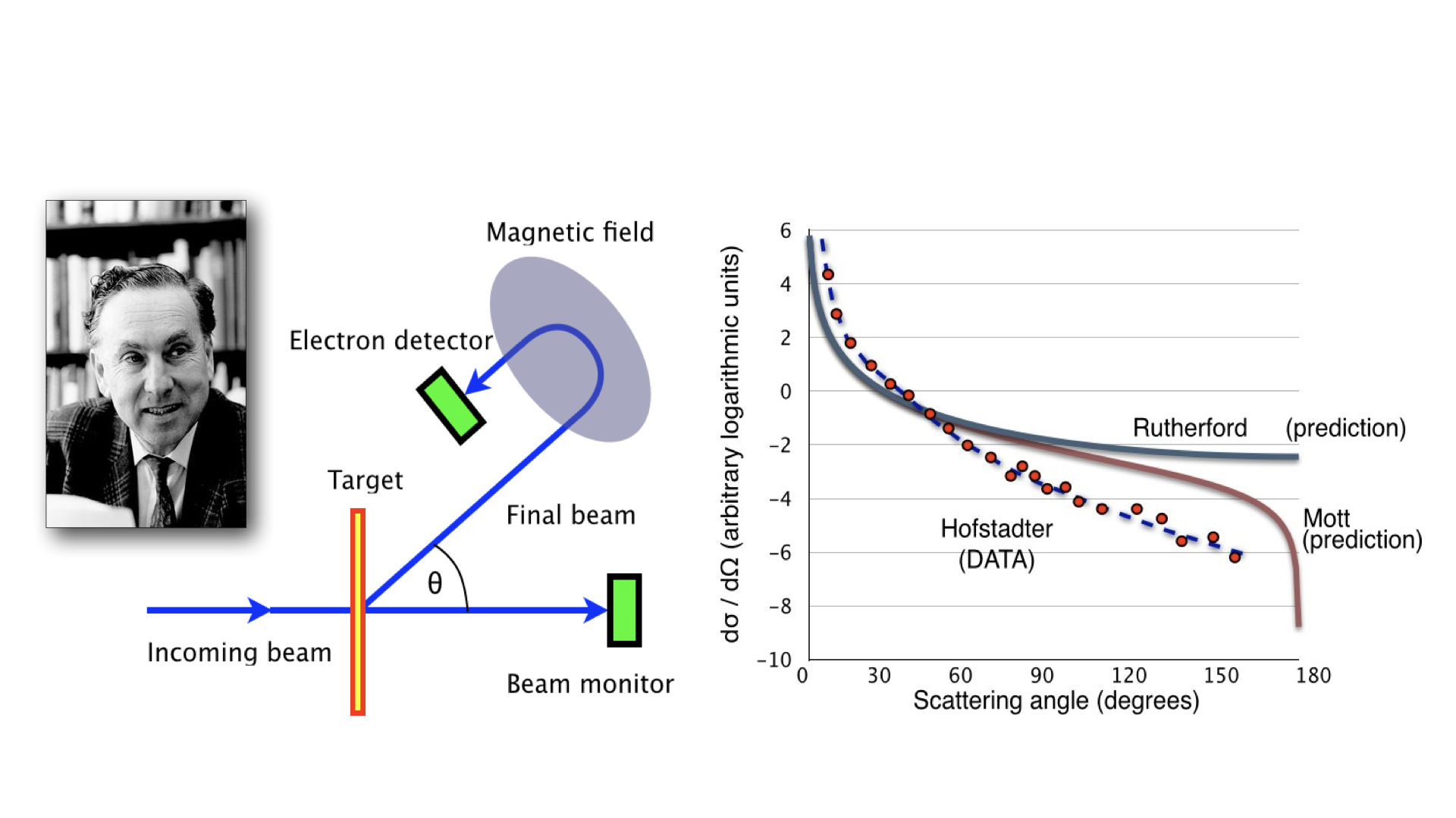
Fig. 1.13 Diagram of the Hofstadter Experiment.

Hofstadter’s experiments provided a strong constraint on the scattering cross-section of nuclei over a broad range of angles. Unfortunately however they showed that that the data still deviates even from the Mott prediction and more is needed to fully describe the nucleus.

This deviation is now interpreted as telling us about the charge/matter distribution in the nucleus. That not only is the nucleus not point-like as assumed in the Mott formula but it has a particular density profile and shape which can be further explicitly probed by electron scattering experiments.