Liquid Drop Model

2. Liquid Drop Model#

Quick Links

Unit 2 : Worked Problems
Unit 2 : Additional Problems
Unit 2 : Equations & Terms
Unit 2 : Flash Cards
Unit 2 : Random Quiz
Unit 2 : Full Quiz
From the Reading List
- Semi-empirical mass formula Martin Chapter 2.3

2.1. Introduction#

So what might the charge and mass distribution be like in Nuclei and how is the Hofstadter experiment interpreted to tell us about it? We know from Rutherford that nucleons in nuclei are likely incompressible. In this unit we’ll see how assuming an incompressible fluid model for the nucleus gives us a simple empirical way to describe some of the features we see in nuclear binding energies. You may already have some exposure to this through studies of the semi-empirical mass formula in year two, but in this course we are going to dig deeper into the reasoning for this model and its strengths and weakness, to justify future extensions.

2.2. Form Factors#

So based on what we saw in the last unit the models assuming scattering of a point source need to be modified if we want to better fit observed data. To factor in the possibility of scattering of a distribution of charges we need to introduce a so called Form-Factor, \(F\), that encompasses information on the structure of the nucleus.

The modified cross-section for a target with a distributed charge distribution can be written as

(2.1)#\[\begin{equation} \left(\frac{d\sigma}{d\Omega}\right)_{\textnormal{distributed}} = |F({\bf q}^{2})|^{2}\times \left(\frac{d\sigma}{d\Omega}\right)_{\textnormal{point-like}}, \end{equation}\]

where \({\bf q}\) is the four-momentum transfer of the interaction, calculated from the incoming electron momentum, \({\bf p}_{1}\), and outgoing electron momentum, \({\bf p}_{2}\), as \({\bf q} = {\bf p}_{1}-{\bf p}_{2}\), \(F\) is our form factor, and the point-like cross-section is our Mott prediction from the previous unit.

To reiterate, a form factor, \(F\), provides additional information on how the distributed structure of the nucleus modifies the interaction probability. Form factors are essentially the Fourier Transform of the density distribution.

(2.2)#\[\begin{equation} F(q) = \int_{-\infty}^{\infty} e^{i~{\bf q} \cdot {\bf r} / \hbar} ~\rho({\bf r})~d^{3} {\bf r} \end{equation}\]

where \(\rho({\bf r})\) is the charge distribution, and \({\bf r}\) is the position. With this relation we can plug in different possible charge distributions of the nucleus and see which one best fits the data. This means detailed measurements of the cross-section over different values of \(\bf q\) allow us to place strong constraints on the the underlying charge distribution itself.

Note

It’s worth pointing out here that the Fourier transform of a delta function is just \(1\), so if the nucleus was indeed a point charge at the center, we would arrive at the same cross-section for a point-like target as before.

Based on our reasoning that the nucleus has some underlying distribution of charge the simplest model we could come up with would be a so called Top-Hat Distribution. That is, constant uniform density, falling to zero at the “edge” of the nucleus. Importantly what was actually found during the early electron scattering experiments was that at higher values of \(\bf q\) we start to see bumps or ridges in our measurements of the cross-section as shown in Fig. 2.1.

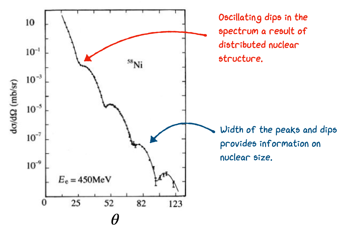
Electron Scattering Form — Fig. 2.1 Measured cross-section from electron scattering of nickel.#

The shape of these structures give an indication of something very close to a top-hat distribution in the center of nuclei, but also that a more “fuzzy” form is needed at the edges. A better fit to the data is given by a so called Saxon-Woods form which accounts for this edge. The Saxon-Woods potential modifies the simple top-hat by introducing a smooth edge parameterized in terms of the radius, \(r\), as follows:

(2.3)#\[\begin{equation} \rho(r) = \frac{\rho_0}{1+{\textnormal{exp}}[\frac{r-a}{d}]} \end{equation}\]

\(a\) is the “edge” of the nucleus defining the width of the top-hat.
\(d\) is the so-called Skin or Surface Thickness.
The same form applies for both the charge and density distribution with slightly different

The plot below shows the charge density versus distance \(r\) from the centre of the nucleus for several known nuclei. We see that as the nuclei size increases the “top-hat” part of the distribution just gets slightly wider but the skin thickness that defines the fall of close to the edge of the nucleus remains mostly constant.

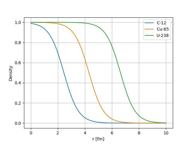
Saxon Woods Form — Fig. 2.2 Saxon Woods charge distribution shape vs Distance from the center of the nucleus for several nuclei.#

Typical Values For the charge density distribution

(2.4)#\[\begin{equation} \rho_{\textnormal{charge}}(r) = \frac{\rho^0_{\textnormal{charge}}}{1+\textnormal{exp}[\frac{r-a}{d}]} \end{equation}\]

\(a = 1.07 A^{1/3} ~\textnormal{fm}~~\textnormal{(radius)}\)
\(d = 0.54~\textnormal{fm}~\textnormal{ (skin thickness)}\)
\(\rho^{0} = 0.06-0.08~e~\textnormal{fm}^{-3}~\textnormal{ (average charge density)}\)
Note: We expect \(\rho^{0}\) to be lower for heavy nuclei as \(Z\) tends away from \(N\).

Typical Values For the mass density distribution

(2.5)#\[\begin{equation} \rho_{\textnormal{mass}}(r) = \frac{\rho^0_{\textnormal{mass}}}{1+\textnormal{exp}[\frac{r-a}{d}]} \end{equation}\]

\(a = 1.2 A^{1/3} ~\textnormal{fm}~~\textnormal{(radius)}\)
\(d = 0.75~\textnormal{fm}~\textnormal{ (skin thickness)}\)
\(\rho^{0} = 0.17~\textnormal{nucleons fm}^{-3}~\textnormal{ (average charge density)}\)

Key observations for both models are:

Modifications are needed between mass distributions and charge distributions due to neutrons having zero-charge.
The parameter values are quite similar in both cases.
The charge radius and mass radius both scale as \(A^{1/3}\).
The central densities are constant, independent of how many nucleons there are in the nucleus.

Studies of electron scattering data found this generally gave a good fit across many nuclei. The last point on central densities is important as it points at a fundamental idea in nuclear physics - the Incompressible Nucleus.

2.3. The Liquid Drop Model#

2.3.1. Introduction#

All the above early studies and information on the nucleus start to lead us towards some basic models to explain the behavior of nuclei. The most basic is the Liquid Drop Model (LDM), based on a description of the nucleus as a drop of “Nuclear Fluid” analogous to a water droplet.

The LDM arises from the following main observations:

Nuclei are spherical (in general) with central density having a fixed value independent of radius. i.e. no matter how many nucleons you pile in to make your nucleus bigger, the density remains the same, the nuclear fluid is Incompressible (like a water drop).
The observation that the radius (size) of the nucleus goes as \(R \sim A^{1/3}\).
The force binding the nucleons together appears to be short range - rather like the intramolecular force in liquids.
The Binding Energy Curve suggests that whatever size of a nucleus, a nucleon situated inside has roughly the same binding energy as all other nucleons. It takes roughly the same energy to free it no matter how many other nucleons are present (neglecting proton/neutron mass differences as we will see later).

These four arguments allow us to build a simple model of the nucleus that satisfies all constraints - The Liquid Drop Model. The assumptions of the model are:

The forces between nucleons are; Repulsive at very short separations, Attractive at separations similar to particle size, and Negligible at larger distances. The collective attraction of nuclei is what keeps them bound together contributing a negative Volume Energy.
The centre of the nucleus is an Incompressible Nuclear Fluid with constant density which is independent of radius, and having a positive Surface Tension Energy. Assuming the fluid is non-rotating, in absence of other forces, the shape adjusts to minimize the surface tension energy resulting in a spherical shape.
If the drop carries Electric Charge then this is uniformly distributed throughout the drop. This combined with the Repulsive Force leads to an additional positive Coulomb Potential Energy in the nucleus.

Putting this together mathematically in the Liquid Drop Model (LDM) leads to an equation for the binding energy for the nucleus as

(2.6)#\[\begin{equation} B(A,Z) = a_{v}A - a_{s}A^{2/3} - a_{c}Z(Z-1)A^{-1/3} \end{equation}\]

In line with our description we have three terms:

\[ \textnormal{Volume Energy Term :}~~ a_{v}A \]

\[ \textnormal{Surface Tension Energy Term :}~~ a_{s}A^{2/3} \]

\[ \textnormal{Coulomb Potential Energy Term :}~~ -a_{c} \frac{Z(Z-1)}{A^{1/3}} \]

Note dividing B(A,Z) by the total nucleons A, gives us a prediction for the binding energy per nucleon plot we discussed in the last set of lectures.

By convention we talk about the binding energy as a positive value (e.g. \(52~\textnormal{MeV}\) for Carbon-12) when in fact it’s a negative value when considering all nucleons in the nucleus - energy needs to be added to the system for us to liberate a nucleon. Our negative volume potential energy term above therefore corresponds to a positive term in the binding energy estimate in the LDM equation.

To understand in a bit more detail the components of the SEMF lets go through them one by one seeing how they improve our fit to real data. We’ll take the data from the IAEA database, and select only the most abundant nuclei with the highest binding energy for each possible value of \(A\). This is how the figures you’ve already seen for binding energy are actually made.

2.3.2. Energy Terms#

2.3.2.1. The Volume Energy Term#

This is the main term, its positive, associated with the short range forces between nucleons pulling them together, its the same for all nucleons (a constant),hence the total for a nucleus is just proportional to the number of nucleons \(A\).

(2.7)#\[\begin{equation} B_{E} \propto A = +a_{v}A ~~~~~~~~ \end{equation}\]

The \(a_{V}\) term sets the scale of the energies we are dealing with in nuclear physics. It is typically given as \(a_{V} = 15.56~\textnormal{MeV}\).

Once the other terms are included (subtracting from this Volume term) we find that a good typical value for the Binding Energy per Nucleon is about \(8~\textnormal{MeV/nucleon}\). We therefore expect the other terms to reduce the binding energy by around \(7-8~\textnormal{MeV}\).

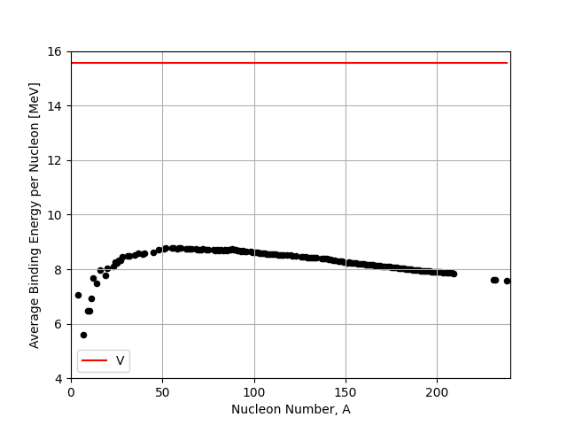
Rutherford Form — Fig. 2.3 Volume term (V) in the liquid drop model compared to the IAEA binding energy data.#

2.3.2.2. The Surface Tension Energy Term#

This is a correction to the Volume Term, subtracting from it, to allow for the assumptions that the outer nucleons near the surface will be less tightly bound. These nucleons make the nucleus weaker, so feel less of the short range attractive forces between nucleons compared to those nucleons well inside the nucleus. It’s like a surface tension term. It’s no surprise then that it is a proportional to the surface area which is proportional to \(A^{2/3}\).

(2.8)#\[\begin{equation} B_{S} = -a_{s} A^{2/3} ~~~~ a_{s} = 17.23 MeV. \end{equation}\]

See here the effect of the surface term. It has the greatest effect on small nuclei, because they have a greater fraction of their nucleons near the surface compared to inside.

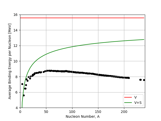
BE Curve with V and V+S terms overlaid. — Fig. 2.4 Volume (V) and Surface (S) term in the liquid drop model compared to the IAEA binding energy data.#

2.3.2.3. The Coulomb Potential Energy Term#

This second correction to the Volume Term comes because nuclei contain positively charged protons that repel each other. This electrostatic repulsion also weakens the nucleus, hence a negative term, reducing the overall binding strength.

By assuming the protons are distributed evenly in the spherical nucleus we can deduce the equation by considering the repulsion of a shell of protons of thickness \(dr\) due to those inside the shell, and integrating over the entire nucleus size.

Recall first that the electric potential energy of a charge \(q_{1}\) in the potential of \(q_{2}\) distance \(r\) away is:

(2.9)#\[\begin{equation} E(r) = \frac{1}{4\pi\epsilon_{0}} \frac{q_{1}q_{2}}{r} \end{equation}\]

The Charge Density (it is uniform remember) is given by :

(2.10)#\[\begin{equation} \rho_{c} = \frac{Q}{V} \approx \frac{3Ze}{4\pi r^{3}_{0}A} \end{equation}\]

Based on this we see that the Electrostatic Energy in the shell \(dr\), we call \(dE_{e}\), is given by:

(2.11)#\[\begin{equation} dE_{e} = \left[{\rho_c \cdot 4\pi r^{2} dr }\right]_{shell} \times \left[ \frac{4\pi r^{3} \rho_{c}}{3} \times \frac{1}{4 \pi \epsilon_{0} r} \right]_{inner} \end{equation}\]

which reduces to

(2.12)#\[\begin{equation} dE_{e} = \frac{4\pi r^{4}\rho_{c}^{2}}{3\epsilon_{0}} dr \end{equation}\]

Integrating this out to the maximum radius of the nucleus, \(r=0\rightarrow R\), gives the total Electrostatic Energy:

(2.13)#\[\begin{equation} E_{e} = \int_{0}^{R} \frac{4}{3} \frac{\pi r^{4}}{\epsilon_0}\rho_{c}^{2}dr = \frac{4}{3} \frac{\pi R^{5}}{5\epsilon_{0}}\rho_{c}^{2} \end{equation}\]

Finally, if we substitute in the charge density given earlier we get

(2.14)#\[\begin{equation} E_{e} = \frac{4}{3} \frac{\pi R^{5}}{5\epsilon_{0}} \frac{Z^{2}e^{2}}{(4/3)^{2} \pi^{2} R^{6}} = \frac{3}{5} \frac{Z^{2}e^{2}}{4\pi \epsilon_{0}R} \end{equation}\]

If we remember that the nuclear size is given by \(R=r_{0}A^{1/3}\) where \(r_{0}\) is the Nucleon Effective Radius and we gather the constants out we get

(2.15)#\[\begin{equation} a_{c} = \frac{3}{5} \times \frac{e^{2}}{4\pi \epsilon_{0} r_{0}} \approx 0.7~\textnormal{MeV} \end{equation}\]

and

(2.16)#\[\begin{equation} B_{C} = -a_{C} \frac{Z^{2}}{A^{1/3}} \end{equation}\]

This is close to our contribution we showed in the equations above, however the analysis includes a slight approximation. As charge is quantized the integration over \(r\) should really only start once a single charge has been enclosed. If this is accounted for the Total Electrostatic Energy is actually given by

(2.17)#\[\begin{equation} B_{C} = -a_{C} \frac{Z(Z-1)}{A^{1/3}} \end{equation}\]

The effect this has on our distribution is shown below. We can see that the coulomb term adds some noise to our prediction as it now depends on \(Z\) and at higher \(A\) the most stable value of \(Z\) can vary slightly from nuclei to nuclei.

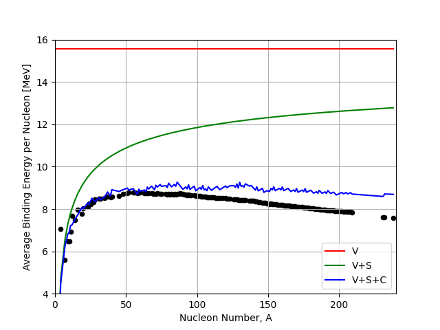
BE Curve with V + S + C terms from LDM overlaid. — Fig. 2.5 Volume (V), Surface (S), and Coulomb (C) terms in the liquid drop model compared to the IAEA binding energy data.#

This change in shape due to the Coulomb Term is of fundamental importance in Nuclear Physics and has profound implications further on in this course. We see that the effect of the Coulomb Term is to bend the B/A curve down at higher A yielding a peak in the B/A curve. One implication concerns the existence of Nuclear Fission in nature.

The gradient of the B/A curve tells us whether energy is released as we move along it. For light nuclei below iron, if nucleons are added to the system for example through fusion, then energy is released.
In contrast however at higher atomic numbers, for example U-235, then energy is only released if nucleons are removed from the nucleus, for example if the nucleus is split up through nuclear fission.

The basic LDM model as stated so far is pretty good but still does not fit the full average binding energy curve very well.

A clue to how to fix this comes from the other important plot shown earlier, the Chart of Known Nuclei.

On a quick look we find two important features:

The most stable nuclei lie roughly on a line where N=Z, nuclei that deviate from this tend to be less stable, (ii) nuclei for which the Z and/or N are an even number tend to be more stable.
Anything that tends to make nuclei less stable, implying the nucleons are less well bound together, is equivalent to lowering the average B/A value - we need to account for this

To do this we introduce two further terms which you may have seen before, the Asymmetry Term and the Pairing Term as follows:

(2.18)#\[\begin{equation} B(A,Z) = a_{v}A - a_{s}A^{2/3} - a_{c}Z(Z-1)A^{-1/3} - \left[a_a(A-2Z)^{2}A^{-1}\right]_{\textnormal{assym}}- \delta_{\textnormal{pair}} \end{equation}\]

At this stage we can regard both these new terms as arising empirically by observation from the data. Though you might guess that the physics origin comes from treating the nucleus using Quantum Mechanics. Note the negative terms - e.g. the more N deviates from the quality with Z, the more negative is the Asymmetry Term and the weaker bound is the nucleus (lower B/A).

2.3.2.4. Nucleon Pairing Term#

Although we can regard the Asymmetry and Pairing Terms as empirical, just an observation that fits the data, we can explain their form better by starting to introduce some Quantum Mechanics (QM). This will lead us later to an improved model of the Nucleus, the Shell Model.

Both protons and neutrons are Fermions, i.e. they have Asymmetric Wave Functions and spin =1/2. Thus they obey the Pauli Exclusion Principle. So we would expect that only two protons (or two neutrons) can occupy a given energy state, one with Spin-up the other Spin-down. In fact the coupling of these spins means it is energetically favorable to have pairs of neutrons or pairs of protons, rather than an odd neutron or proton alone in a given level.

In the figure below each line corresponds to a new energy level that the protons or neutrons can occupy when the states below them are filled.

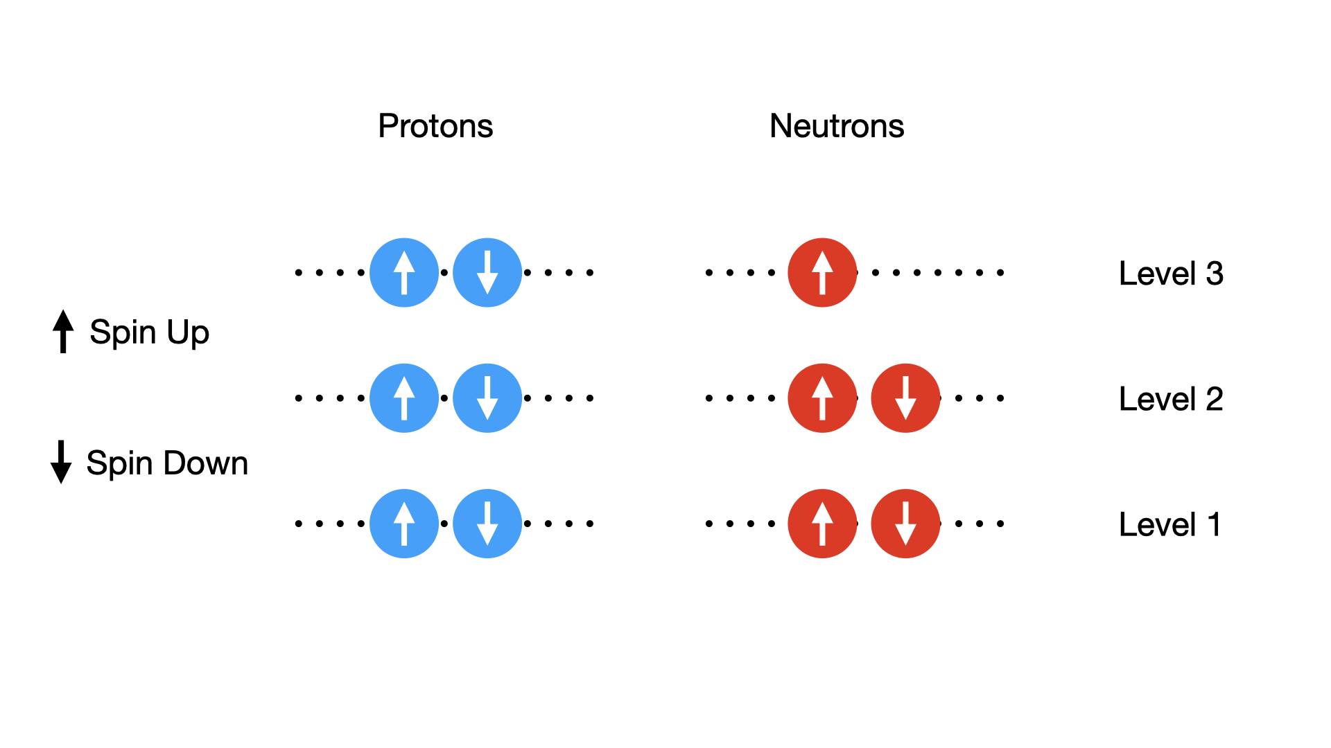
Nucleon pairing diagram showing protons and neutron spin alignment. — Fig. 2.6 Possible pairing states of protons, each possible energy state or ‘level’ can have two protons or neutrons inside it, provided their spins are opposite.#

We might expect that the neutrons and protons in a nucleus might best pile into energy levels in pairs. If each sequential level has a higher energy this would allow most nucleon to be in the lowest energy levels as possible and would be the most stable configuration. Based on this simple pairing idea there are three possible states

Even-Even Even numbers of protons and even numbers of neutrons would therefore yield the largest positive contribution to the binding energy. This is referred to as an Even-Even configuration.
Even-Odd If we have a single left over proton, or a single left over neutron, we end up with only one partially filled energy level on the neutron or proton side. This is referred to as an Odd-Even state and as a result the nucleus is less bound and it is a state of intermediate stability. This is because the unpaired nucleon is not tightly bound.
Odd-Odd Finally we can consider states where both an odd proton and an odd neutron is left. These are referred to as Odd-Odd states. Because they are the least stable they are very rare in nature.

So how nucleons pair up is important in the binding energy and this dictates the \(\delta_{pair}\) term.

(2.19)#\[\begin{split}\begin{align} \delta_{\textnormal{pair}} &= +a_{p}A^{-1/2} ~~~~\textnormal{for N odd AND Z odd}\\ \delta_{\textnormal{pair}} &= 0 ~~~~~~~~~~~~~~~~~~~\textnormal{for N even OR Z even} \\ \delta_{\textnormal{pair}} &= -a_{p}A^{-1/2} ~~~~\textnormal{for N even AND Z even}\\ \end{align}\end{split}\]

Note the negative term in the binding energy equation that cancels out the negative term in the Even-Even case to produce an increase in binding energy overall (the nucleus is more stable). The \(A^{-1/2}\) part is an empirical fit and the \(a_p\) factor is a constant. Its important to get the sign of the term correct.

2.3.2.5. Nucleon Assymetry#

Finally we also see that nuclei are also more stable, roughly, if there are qual numbers of neutrons and protons (and preferably in pairs, Even-Even).

In the simplest QM Model (an infinite 3d potential well) we can assume that spacing between the energy levels is a constant value and is proportional to the inverse of the volume hence \(\Delta E \propto A^{-1}\). A full derivation of this is beyond us at this point but if we were to do so it would yield the form

(2.20)#\[\begin{align} B_{A} = -a_{a} (A-2Z)^{2}A^{-1} \end{align}\]

where \(a_{a}\) is another constant. Importantly this gives zero if \(N=Z\) as then \(A=2Z\).

If we look at how both the additional pairing and asymmetry terms in our model behave we see that they are capable of bringing us closer to the data.The asymmetry term makes the biggest difference at high \(A\) whilst the pairing term brings us slightly closer at low \(A\) and has smoothed out the fluctuations we saw at higher atomic mass. We can now predict the binding energies for most of the common nuclei to within a few percent which is not bad for still a relatively simple model!

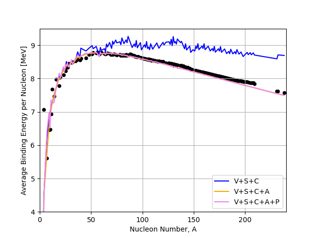
ldm_combined — Fig. 2.7 Volume (V), Surface (S), Coulomb (C), Asymmetry (A), and Pairing (P) terms in the liquid drop model compared to the IAEA binding energy data.#

2.4. Total Liquid Drop Binding Energy Equation#

With all our terms added together we finally have a

(2.21)#\[\begin{align} B(A,Z) = a_{v} A - a_{s}A^{2/3} - a_{c} Z(Z-1) A^{-1/3} - a_{a}(A-2Z)^{2}A^{-1} + \delta \end{align}\]

or in terms of B/A for the plots above

(2.22)#\[\begin{align} B(A,Z)/A = a_{v} - a_{s}A^{-1/3} - a_{c} Z(Z-1) A^{-4/3} - a_{a}(A-2Z)^{2}A^{-2} + \delta A^{-1} \end{align}\]

where

\(a_{v} = 15.5 \textnormal{MeV}\),
\(a_{s} = 16.8 \textnormal{MeV}\),
\(a_{c} = 0.72 \textnormal{MeV}\),
\(a_{a} = 23.0 \textnormal{MeV}\),
\(a_{p} = 12.0 \textnormal{MeV}\).

Clarification.

In several definitions you will find online and in text books the definition of the delta term and whether it is plus or minus in the top level equation will change. As we discussed in the lecture even here it is swapped relative to what was above. The key thing we need to remember is that EVEN-EVEN nuclei are more stable and therefore they should always increase the binding energy.

Whilst emperical in its form this is an amazing useful equation as it allows us to make estimates of the energies of radiative emissions. For example, let’s say we consider a nuclear reaction such as alpha decay

\[ ^{230}Th \rightarrow ^{226}Ra + \alpha \]

We can use the SEMF to calculate the total rest energy of each component object in MeV, and what we find is that there is a mass deficit which ends up being distributed between the daughter nuclei and the alpha particle in the form of kinetic energy. Due to conservation of momentum the alpha particle carries away most of this energy so our liquid drop model can be used to estimate the energy of alpha decay emissions for different nuclei.

2.5. Conclusion#

The Semi Empirical Mass Formula or Binding Energy Equation gives an excellent fit to the overall shape of the Binding Energy Curve and starts to give us the basis of a model for nuclei and how they behave. However, it has its failings. In Summary:

SEMF Advantages

It makes good predictions of the masses and binding energies of most nuclei and explains the basic shape of the Binding Energy (BE) Curve.
It allows predictions of the energy release in nuclear decay (or energy input needed to make a reaction occur)
It suggests, for instance, why fission can occur in nature due to changes in the binding energy for fission parents and daughters.

SEMF Disadvantages

It does not explain why there are spikes in the BE curve at certain nuclei.
It doesn’t explain nuclei shape, in particular why some are observed to not be spherical.
It doesn’t explain nuclear properties like Nuclear Spin, Parity, and Magnetic Moment.

Later on in this course we’ll see how the SEMF is suitable for doing a lot of different radioactive decay and fusion/fission calculations, but in the next topic instead we’ll try to address some of these underlying weaknesses of the model to better understand the true nature of the nucleus.