1. Stream A Introduction

In this first session, we revise functions, their visualisation and the behaviour of some of the most commonly used functions in physics. In future sections we will explore the diferentiation of functions and how we can approximate functions using series expansions. A flavour of what these tools enable is shown in Fig. 1.1.

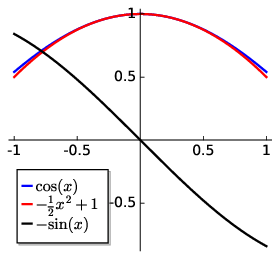
Fig. 1.1 The function \(f(x) = \cos x\) corresponds to the blue curve. The slope of the function, which is obtained by differentiation, corresponds to the function \(-\sin x\). Near \(x = 0\), \(f(x) = \cos x\) can be approximated by a polynomial using a series expansion. The tools of differentiation and series expansion will be introduced in subsequent sections.

Functions are the primary tools of the mathematical description of the physical world. The simplest functions are those defined as in terms of a single variable such as \(x\) notated as \(f(x)\), or ‘f of x’. In physics, we are often looking to determine some unknown function, such as how does position vary with time for a particle experiencing constant acceleration? What is mathematically meant by a function?

A function is a process of association. In maths, we can associate numbers from one set to another. In physics, we can associate values of position with values of time. Mathematically, the association of an output to an input is often, but not always, unique; i.e., a given input produces a single output. Functions are powerful since they enable us to make predictions.

The notation used in mathematics typically has the form \(y=f(x)\). Since there is just a single input, \(x\), this is a one dimensional (1D) function. A 2D function takes the form \(z=f(x,y)\) and so on. What exactly the function \(f\) is can then be defined in terms of the input variables, constants and indeed other functions.

There are a number of common terms to describe functions. Since \(y\) is dependent on \(x\), it is referred to as the dependent variable, whilst the input \(x\) is referred to as the independent variable. All values of the input which produce a defined output is referred to as the domain of the function.

For example, if we insist on the output being a real number, then the domain of the function \(f(x)=\sqrt(x)\) corresponds to positive, real numbers, since the square root of a negative number is not a real number. Similarly, if the output for a particular input has no well defined value, then that input value is not part of the domain of the function. For example, \(f(x)=1/x\) does not have a well defined output for \(x = 0\); hence, the input value, \(x = 0\) is not part of the domain of the function. The corresponding values of the output are referred to as the range of the function.

Visualising functions can provide us with an intuitive understanding of the physical behaviour. In physics, we focus mostly on graphing functions: the domain is typically on the horizontal axis and the range on the vertical axis. The function can then be visualised as a 1D curve of these \(x,\,\,y\) points. Such visual graphs are also very useful in performing analysis of function such as how the function changes (i.e. differentiation).

1.1. Explicit functions

Explicit functions are those that we encounter most frequently. Some of the more frequently occurring functions in physics are shown in Table 1.1.

Table 1.1 Basic maths functions

Name	Function
Polynomial	\(y=a_{0}+a_{1}x\)
Power law	\(y=x^{a}\)
Exponential	\(y=a^{x}\)
Logarithm \(^{x}\)	\(y=\log_{a}x\)
Trigonometric	\(\cos x\), \(\sin x\), \(\tan x\)

1.1.1. Polynomial functions

These take the form:

(1.1)\[ y=a_{0}+a_{1}x+a_{2}x^{2}+a_{3}x^{3}+...+a_{n}x^{n} \]

Polynomials are defined by the highest power or degree. For example:

• Linear: \(y=13x-2\) has degree of 1

• Quadratic: \(y=x^{2}-4x+1\) has degree of 2

• Cubic: \(y=x^{3}+x-3\) has degree of 3

and so on as visualised in Fig. 1.2.

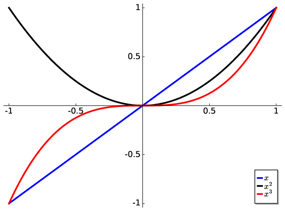
Fig. 1.2 Examples of polynomial functions with linear, quadratic and cubic.

1.1.2. Exponential and Log functions

The exponential function occurs frequently in the description of physical phenomenon

(1.2)\[ y=e^{x} \]

Its special place in physics arises from the property that the slope of the curve is the same function. We will explore this again when we explore differentiation. We refer to \(x\) as the exponent. The sign of the exponent determines if the function describes exponential decay, \(y=e^{-x}\), or exponential increase, \(y=e^{+x}\).

The natural logarithmic function is the inverse of the exponential function and is denoted as:

(1.3)\[ y=\log_{e}x = \ln x \]

\(e\) demotes the base of the logarithm. The base can be any number, although in physics we most commonly encounter the base \(e\), or the natural, logarithm, or the base \(10\) logarithm. The function \(y=\log_{10}x\) is the inverse of \(y=10^x\).

If we start with the equation \(y=x^a\) it follows that \(\log_a y = x\) where the notation \(\log_a\) means \(\log\) to the base \(a\) (for \(a>1\)). We often use the notation \(\log_e = \ln x\) for the natural logarithm, but note that programming languages (e.g. Matlab and Python use \(\log(x)\) to denote the natural logarithm of \(x\), and \(\log10(x)\) to denote the base 10 logarithm of \(x\).

1.1.3. Logarithm Rules

There are some rules of logarithms that you should be completely familiar and at ease with:

\[\begin{split} \begin{aligned} \log_a x + \log_a y &= \log_a (xy)\\ \log_a x - \log_a y &= \log_a \left(\dfrac{x}{y}\right)\\ n\log_a x &= \log_a x^n\\ \log_a 1 &= 0\\ \log_a x &= \dfrac{\log_b x}{\log_b a}\end{aligned} \end{split}\]

where \(x\) and \(y\) are any positive number and \(b>1\).

1.2. Implicit functions

To illustrate what is meant by an implicit function, consider the equation for a circle:

(1.4)\[ x^{2}+y^{2}=1 \]

What is \(f(x)\) here? For such implicit equations, we have to coax out the function or functions. We do this by solving the equation for the dependent variable \(y\). In the case of the circle equation, first subtract \(x^2\) from the left and the right hand sides of the equation:

(1.5)\[ y^{2}=1-x^{2} \]

and then take the square root of both sides:

(1.6)\[ y =\pm\sqrt{1-x^{2}} \]

The symbol \(\pm\) tells us that both positive and native values are solutions, and since we want our functions to map an input to a unique output, the explicit functions relating the input, \(x\), with the output, \(y\), are then

(1.7)\[\begin{split} \begin{aligned} f(x) & =\sqrt{1-x^{2}}\\ g(x) & =-\sqrt{1-x^{2}}\end{aligned} \end{split}\]

These are the positive and negative semi-circles as shown in Fig. 1.3.

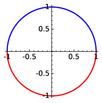
Fig. 1.3 The equation for a circle is not an explicit function. Instead it is comprised of two implicit functions defining two semi-circles.

1.3. Parametric functions

Another type of implicit function is when two, or more, variables are dependent on some other variable. For example, we might have two functions \(x=f(t)\) and \(y=g(t)\). Due to this extra dependency on the parameter \(t\), these are referred to as parametric functions.

An example of the use of parametric functions in physics are the kinematic equations for motion in 2D which describe the position of particle in the \(x\) and the \(y\) directions as a function of time \(t\):

\[\begin{split} \begin{aligned} x(t) & =x_{0}+v_{x_{0}}t+\frac{a_{x}}{2}t^{2}\\ y(t) & =y_{0}+v_{y_{0}}t+\frac{a_{y}}{2}t^{2}\end{aligned} \end{split}\]

The path that the particle follows as \(t\) is varied is shown in Fig. 1.4.

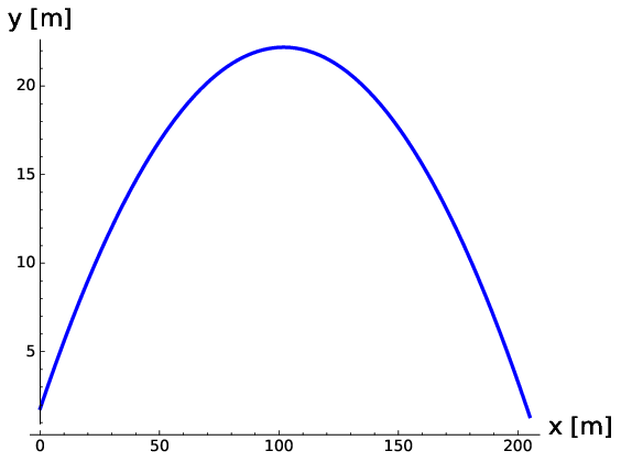
Fig. 1.4 An example of parametric equations in physics are the kinematic equations of motion. Here we calculate the \(x,y\) spatial variables as a function of time \(t\) for some object with initial speed \(v_{x_{0}},v_{y_{0}}=50,20\) m/s. In this example, the variable for time, \(t\), is the ‘parameter’ which both \(x,y\) are dependent upon.

1.4. Continuous and discontinuous functions

Continuous functions are those for which \(y\) vary smoothly without sudden ‘jumps’ when the value of \(x\) is varied. Discontinuous functions have breakages such as when the function has no value or goes to infinity. Simple examples of discontinuous functions are of the form \(1/x^{n}\), these break down as we approach \(x=0\) as shown in Fig. 1.5. The trigonometric function \(\tan x\) breaks down repeatedly at \(x=\pi/2,\,\,3\pi/2..\) where it goes to infinity.

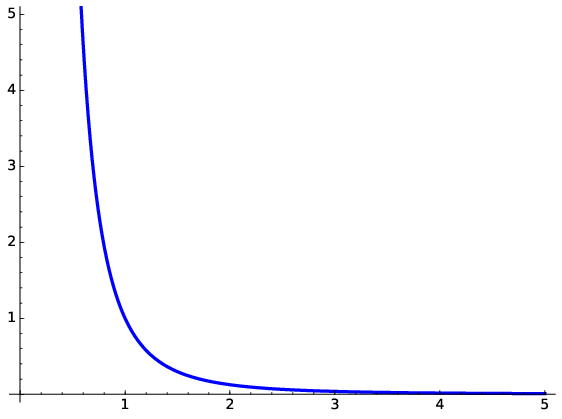
Fig. 1.5 Examples of discontinuous functions; \(x^{-3}\) goes to infinity as \(x\rightarrow0\).

1.5. Asymptotes

An asymptote of a function is a horizontal or a vertical line that the curve of the function approaches, but never reaches, as it tends towards infinity. As an example, consider again the function \(f(x)=\tan x\). This has vertical asymptotes, shown as dashed lines in Fig. 1.6, at \(x=\pi/2,\,\,3\pi/2\) and so on. The function \(f(x)=1/x\) has a vertical asymptote at \(x = 0\) and a horizontal asymptote at \(y = 0\).

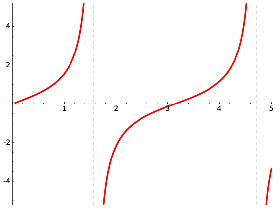
Fig. 1.6 Examples of discontinuous functions; \(\tan x\) is periodically discontinuous at every odd multiple of \(\pi/2\). Vertical asymptotes are shown for \(\tan x\) as dashed lines.

Note

Defining Domains - Added 10/10/24

When defining the ranges of a function we use the asymptotes to define the edges of validity. For example a function with an asymptote at \(x=0\) but that is valid for all other regions would say to have the domain

\[ x \rightarrow [-\infty,0] , [0,\infty] \]

A common notation is round brackets are used if the limit value is also valid e.g. \(x \rightarrow (-1,0)\) for both limit values valid or \(x\rightarrow (-1,\infty]\) or \(x\rightarrow [-\infty,-1)\) if just one limit is valid.

In this course as long as you understand where the limitations of a function may be and understand how to find them for unseen functions, then that is enough.

Note

Horizon Asymptotes - Added 10/10/24

When determining horizontal asymptotes there is a standard rule to estimate the presence of one when given fractions which include polynomials on the top on the bottom.

For example take the function

\[ f(x) = \frac{Ax^{2} + x + 8}{2x + 4} \]

Here the numerator polynomial has a rank of two (it’s highest power is \(x^{2}\)), whilst the denominator has a rank of one (it’s highest power is \(Bx^{1}\)).

We can find the rank of any of the polynomials we are given in this form, and determine the rank of the numerator, \(n\), and the denominator \(d\).

The presence of a horizontal asymptote is then determined by

• \(n > d\) There is no horizontal asymptote

• \(n == d\) There is one horizontal asymptote at \(y = A/B\).

• \(n < d\) There is one horizontal asymptote at \(y=0\).

1.6. Symmetry

Another useful property of a function is its symmetry for positive and negative \(x\). For example, if \(f(-x)=f(x)\), then the function is referred to as even. If \(f(-x)= -f(x)\), then the function is described as odd. It is easy to appreciate this by visualising the function and checking if it is symmetric with respect to the \(y\)-axis or the origin. The symmetry is easy to appreciate via graphs such as in Fig. 1.7 and Fig. 1.8.

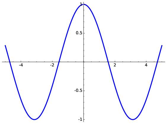
Fig. 1.7 Even and odd functions are defined if there are symmetric around the \(y\)-axis or origin respectively; an even function such as \(\cos x\) is symmetric around the \(y\)-axis.

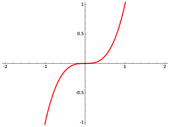
Fig. 1.8 Even and odd functions are defined if there are symmetric around the \(y\)-axis or origin respectively; an odd function such as \(x^{3}\) has rotational symmetry with respect to the origin, meaning that its graph remains unchanged after rotation of 180\(^{\circ}\) about the origin.

1.7. The inverse of a function

For a typical function, we can map values of \(y\) to \(x\) using \(y=f(x)\). Often we may wish to reverse this process and map values of \(x\) to values of \(y\). This is usually straight forward via:

1. Transpose the equation \(y=f(x)\) by solving for \(x\).

2. Swap \(y\) with \(x\) in the transposed equation.

3. Replace \(y=\) with \(f^{-1}(x)\)

4. Note that the inverse function \(f^{-1}(x)\) is not the same as \(1/f(x)\).

To illustrate this, consider the example of \(y=f(x)=x^{3}\):

1. Transpose the equation \(y=x^3\) by solving for \(x\): \(x=y^{\frac{1}{3}}\).

2. Swap \(y\) with \(x\) in the transposed equation: \(y=x^{\frac{1}{3}}\).

3. Replace \(y=\) with \(f^{-1}(x)\): \(f^{-1}(x) =x^{\frac{1}{3}}\).

4. Note that the inverse function \(f^{-1}(x) =x^{\frac{1}{3}}\) is not the same as \(1/f(x)=x^{-3}\).

As shown in Fig. 1.9, the function and its inverse have a symmetry. Another way to think above inverse functions is to visualise \(f(x)\) and then reflect it through a \(45^{\circ}\) line in the \(x,\,y\) plane.

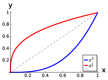
Fig. 1.9 When visualised the inverse of a function will be its reflection through a 45\(^{\circ}\) line. The axis labels will swap such that for the inverse function \(y\) will be on the horizontal. The inverse function effectively enables us to determine a value of \(x\) for a given \(y\).