5. Power and Maclaurin Series

5.1. Approximating functions using series

We can already see how higher derivatives can enable functions to be analysed for critical points including maxima and minima. Another, even more powerful application of higher derivatives is approximating functions as polynomials. This is really useful because the resulting polynomials, although approximate, are often much easier to study and evaluate than the original functions. Applied to physics, this approach enables complicated analytical expressions to be simplified. Hence, whenever you are attempting to solve some complex physical model, series approximations can reduce the work involved and may ultimately enable predictions or deeper insights to be made.

5.2. Power series

An infinite power series about some point \(x=c\) is defined as

\[ f(x)=a_{0}+a_{1}(x-c)^{1}+a_{2}(x-c)^{2}+\cdots=\sum_{n=0}^{\infty}a_{n}\left(x-c\right)^{n} \]

Typically, \(c\) represents a point near to which we are particularly interested in knowing the behaviour of the function. Often in physics, we try to choose our coordinate system, or independent variable, such that \(c = 0\).

Having defined a power series, we now show that we can rewrite functions by relating the coefficients \(a_n\) to the appropriate order of derivative of \(f(x)\) evaluated at \(x=c\). Consider the 3rd order polynomial

\[ f(x) = a_0+a_1(x-c)+a_2(x-c)^2+a_3(x-c)^3 \]

Note firstly that we have \(a_0=f(x=c)\). The first three derivatives are:

\[\begin{split} \begin{aligned} \frac{df}{dx}\equiv f^{(1)}&=a_1+2a_2(x-c)+3a_3(x-c)^2 \\ \frac{d^2f}{dx^2}\equiv f^{(2)}&=2a_2+2 \cdot 3a_3(x-c) \\ \frac{d^3f}{dx^3}\equiv f^{(3)}&=2 \cdot 3a_3 \\ \end{aligned} \end{split}\]

Hence we can see that the \(n\)^th^ coefficient in the polynomial corresponds to the \(n\)^th^ derivative evaluated at \(x=c\); i.e.,

\[\begin{split} \begin{aligned} f^{(0)}(x=c)&=a_0\\ f^{(1)}(x=c)&=a_1\\ f^{(2)}(x=c)&=2a_2 \\ f^{(3)}(x=c)&=2 \cdot 3a_3 \\ f^{(4)}(x=c)&=2 \cdot 3 \cdot 4 a_4 \\ \end{aligned} \end{split}\]

We could repeat this process for a higher order polynomial to find the general result that

\[ a_n=\frac{1}{n!}f^{(n)}(x=c) \]

so that

\[\begin{split} \begin{aligned} f(x)&=a_{0}+a_{1}(x-c)^{1}+a_{2}(x-c)^{2}+\cdots \\ &=\sum_{n=0}^{\infty}a_{n}\left(x-c\right)^{n} \\ &=\sum_{n=0}^{\infty}\frac{1}{n!}f^{(n)}(x=c)\left(x-c\right)^{n} \end{aligned} \end{split}\]

where the factor \(1/n!\) arises from the repeated differentiations which reduce the power by one each time as we saw above for the 3rd order polynomial.

If the function \(f(x)\) is a polynomial, the final relation above is exact for all values of \(x\). However, we can generalise the techniques to find approximate expressions to more complex functions. We are able to do this due to the \(1/n!\) prefactor such that higher order terms might become increasingly small as long as the higher order derivatives also become increasingly small. Such an approximation is referred to as a Taylor series.

5.3. Taylor series centred at zero

This special case is often referred to as a Maclaurin series. It takes the form

\[ f(x)=\sum_{n=0}^{\infty}\frac{f^{(n)}(0)x^{n}}{n!} \]

Writing the first \(n\) terms, we create a \(n\)-degree polynomial of the form:

\[ f(x)\approx\frac{1}{0!}f^{(0)}(0)x^{0}+\frac{1}{1!}f^{(1)}(0)x^{1}+\frac{1}{2!}f^{(2)}(0)x^{2}+\frac{1}{3!}f^{(3)}(0)x^{3}\ldots+\frac{1}{n!}f^{(n)}x^{n} \]

The key ingredient here is the specific function \(f\) we are attempting to approximate. We need to calculate the value of this function and its derivatives at \(x=0\). By doing so, we are then able to approximate the function for \(x \ne 0\).

5.3.1. Example 1: The exponential series

The easiest example to start with is the function \(e^{x}\), since its derivatives all equal the function itself. Here we expand the series to a 4\(^{\mathrm{th}}\) degree polynomial:

\[ e^{x}\approx e^{0}+e^{0}x+\frac{e^{0}}{2}x^{2}+\frac{e^{0}}{6}x^{3}+\frac{e^{0}}{24}x^{4} \]

and since \(e^{0}=1\), we have:

\[ e^{x}\approx1+x+\frac{x^{2}}{2}+\frac{x^{3}}{6}+\frac{x^{4}}{24} \]

As shown in Fig. 5.1, this simple approximation is accurate up to \(x\approx 2\) and diverges afterwards.

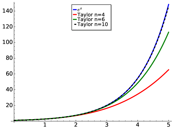
Fig. 5.1 The Taylor approximation of \(e^{x}\) is shown as a 4th degree, 6th degree and 10th degree polynomial.

We can improve the approximation by adding more higher order terms. Since we can see the form of the series as:

\[ e^{x}=\sum_{n=0}^{\infty}\frac{x^{n}}{n!} \]

adding more terms is simple, so a 6-degree polynomial approximation is:

\[ e^{x}\approx1+x+\frac{x^{2}}{2}+\frac{x^{3}}{6}+\frac{x^{4}}{24}+\frac{x^{5}}{120}+\frac{x^{6}}{720} \]

5.3.2. Example 2: The Binomial series

Binomial functions are of the form

\[ f(x)=(1+x)^{k} \]

which can be expanded by performing a Taylor approximation centred at \(x=0\). The first three derivatives are:

\[\begin{split} \begin{array}{ll} f^{(0)}(x)=(1+x)^{k} & f^{(0)}(0)=1\\ f^{(1)}(x)=k(1+x)^{k-1} & f^{(1)}(0)=k\\ f^{(2)}(x)=k(k-1)(1+x)^{k-2} & f^{(2)}(0)=k(k-1)\\ f^{(3)}(x)=k(k-1)(k-2)(1+x)^{k-3} & f^{(3)}(0)=k(k-1)(k-2) \end{array} \end{split}\]

Hence, the series is:

\[\begin{split} \begin{aligned} f(x) & =f^{(0)}(0)x^{0}+\frac{1}{1!}f^{(1)}(0)x^{1}+\frac{1}{2!}f^{(2)}(0)x^{2}+\frac{1}{3!}f^{(3)}(0)x^{3}+\cdots\\ & =1+kx+\frac{k(k-1)x^{2}}{2}+\frac{k(k-1)(k-2)}{6}x^{3}+\cdots\end{aligned} \end{split}\]

The binomial series is a useful analytical tool. For example, when both \(|x|\ll1\) and \(|nx|\ll1\) than we use just the first two terms in the expansion:

\[ (1+x)^{k}\approx1+kx \]

You will see this applied in many cases in your physics courses where approximations can be made for certain limiting conditions.

The total energy derived from the theory of special relativity is \(E=mc^{2}(1-v^{2}/c^{2})^{-\frac{1}{2}}\).

For \(v << c\), this can be simplified using a binomial expansion of \((1+x)^k\): The quantity \(-v^{2}/c^{2}\) corresponds to \(x\) and \(k=-\tfrac{1}{2}\).

For \(x << 1\), \((1+x)^{k}\) approximates to \((1+\tfrac{1}{2}x)\). Hence

\[\begin{split} \begin{aligned} E & =mc^{2}(1-v^{2}/c^{2})^{-\frac{1}{2}}\\ & \approx mc^{2}(1+\tfrac{1}{2}v^{2}/c^{2})\\ & =mc^{2}+\tfrac{1}{2}mv^{2}.\end{aligned} \end{split}\]

When we then multiple the constant \(mc^{2}\) term, we can discover that the classical form of kinetic energy appears in the low speed limit of special relatively.