3. Differentiation

Once we are comfortable recognising and using different functions, a key next step is analysing them to determine their rate of change. This type of analysis is referred to as differential calculus. The rate of change, or derivative, can be used to determine quantities such as the slope of the function at specific values of input. If we repeat this process we may obtain the rate of change of the derivative which can enable us to determine local points of maxima, minima or even inflection. This power to describe how variables change with each other was instrumental in the development of physics and will be a key component in your analytical toolbox.

3.1. Rates of change

The rate of change of some function corresponds to the slope of the curve of the function. As a first approximation, we can determine the slope at a point \(x_{1}\) by considering how much the value of the function differs compared to another point \(x_{2}\). This is approximate if the variation of the function between the two points is not a straight line. If, for these two values of input, the corresponding outputs of the function are \(y_{1}\) and \(y_{2}\), respectively, then the slope corresponds to the change in \(y\) relative to the change in \(x\):

\[\mathrm{slope}=\frac{y_{2}-y_{1}}{x_{2}-x_{1}}=\tan\theta\]

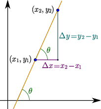
Fig. 3.1 The rate of change of some function corresponds to the slope of the curve of the function. As a first approximation, we can determine the slope at a point \(x_{1}\) by considering how much the value of the function differs compared to another point \(x_{2}\). This is exact if the variation of the function between the two points is a straight line, otherwise it is an approximation.

As you can see from Fig. 3.1 the slope or gradient is the ratio of opposite to the adjacent which corresponds to the trigonometretic function \(\tan(\theta)\), which is why we often refer to the slope as the tangent to the the function. Typical notation uses the Greek letter delta (\(\delta,\,\Delta\)) for increment or difference in values of variable such as \(\delta x\). Hence the rate of change is:

\[ \mathrm{slope}=\frac{\delta y}{\delta x}=\frac{y_{2}-y_{1}}{x_{2}-x_{1}} \]

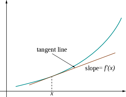
Fig. 3.2 The derivative of a function at a point \(x\) can be illustrated with as the tangent

As long as we choose a small enough increment of \(\delta x\), this method of finding the slope works well even for functions that do not vary linearly. We can take this further by choosing this increment such that it approaches the limiting value of zero, which we denote as \(\delta x\rightarrow0\). Noting that \(y_1 = f(x_1)\) and \(y_2=f(x_2)=f(x_1+\delta x)\), the derivative becomes in the limit of \(\delta x\rightarrow0\)

(3.1)\[ \lim_{\delta x\to0}\frac{\delta y}{\delta x}=\frac{f(x+\delta x)-f(x)}{\delta x} \]

This turns out to be such a useful quantity in physics that we replace the notation

\[ \lim_{\delta x \to 0}\frac{\delta y}{\delta x} \]

with

(3.2)\[ \frac{dy}{dx} \]

which we refer to as the rate of change of \(y\) with \(x\). Hence we have,

(3.3)\[ \frac{dy}{dx}=\frac{f(x+\delta x)-f(x)}{\delta x} \]

We can use equation to determine the rate of change of any function. For example, consider the quadratic function \(f(x)=3x^{2}+2\), for which we have,

\[\begin{split} \begin{aligned} f(x+\delta x) & =3[(x+\delta x)^{2}]+2\nonumber \\ & =3[x^{2}+2x\delta x+(\delta x)^{2}]+2\nonumber \\ f(x+\delta x)-f(x) & =6x\delta x+3(\delta x)^{2}=\delta y\nonumber \end{aligned} \end{split}\]

Hence $\( \begin{aligned} f(x+\delta x)-f(x) =6x\delta x+3(\delta x)^{2}=\delta y\nonumber \end{aligned} \)$

Once we have the change \(\delta y\), we can determine the rate of change by using eq.

\[\begin{split} \begin{aligned} \lim_{\delta x\to0}\frac{\delta y}{\delta x} & =\frac{6x\delta x+3(\delta x)^{2}}{\delta x}\label{diff2}\\ \lim_{\delta x\to0}\frac{\delta y}{\delta x} & =6x+3\delta x = 6x\nonumber \\\end{aligned} \end{split}\]

The last step, where we eliminate the term \(3\delta x\), is what we mean by taking \(\delta x\) to be small enough. This technique of considering what happens when the difference between two points approaches zero is something that we make a great deal of use of in deriving mathematical descriptions of the physical world. As you can see the end result for the slope is now independent of the value of \(\delta x\), in other words for small enough differences between points the slope does not depend on the difference. Hence the slope becomes a property of the value of the input point alone. Finally we have

(3.4)\[ \frac{dy}{dx} =6x=f'(x) \]

where \(dy/dx\) represents the instantaneous rate of change of the function. On the right hand side of eq. we have introduced the notation \(f'(x)\), where the prime, \((')\), after the \(f\) tells us that this is the first differential of \(f\) with respect to the input variable, which in tis case is \(x\). There are a variety of notation styles for the derivative of a function that you will encounter:

\[ \frac{df}{dx}=\frac{d}{dx}f(x)=f'(x)=y'=\frac{dy}{dx} \]

which all mean the same.

In Fig. 3.3, we see both the function and its derivative visualised allowing us a more intuitive understanding of the meaning of differentiation.

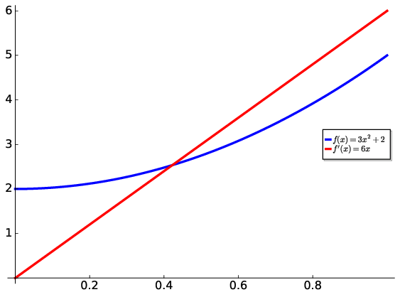
Fig. 3.3 Differentiation is an analysis of the instantaneous rate of change in a function. Here in the example of \(f(x)=3x^{2}+2\) the derivative is determined as \(f'(x)=6x\). Notice, this is a constant rate of change. The process effectively associates a \(x^{2}\) function to a \(x^{1}\) function. More generally, we can say it is a mapping from \(x^{n}\) to \(nx^{n-1}\).

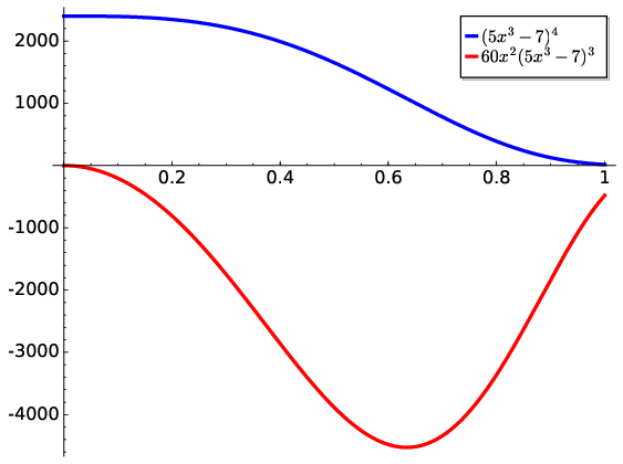
Fig. 3.4 An example of a composite function in the form of \(y=f(g(x)\) and its derivative \(y'\). The latter can be derived analytically using the chain rule. The rate of change is all negative in this domain of \(x\) with a minimum near \(x=0.63\)

3.2. Rules of differentiation

In our example above, from Eq. -, we used around 6 steps to go from \(f(x)\) to \(f'(x)\). This is referred to as differentiation from first principles. Once we determine this for standard functions, we can switch to using shorthand ‘rules’ for our standard derivatives such as those listed in Table 1.1.

Table 3.1 Differentiation Rules : As we tend to work with many standard functions, their derivatives tend to be familiar and become memorised. These of course can all be derived from first principles. Notice, in the case of exponential, its derivative is itself!

Type	Function	Derivative
Constant	\(c\)	0
Power	\(x^{n}\)	\(nx^{n-1}\)
Exponential	e\(^{x}\)	e\(^{x}\)
Log	\(\ln x\)	\(\frac{1}{x}\)
Cosine	\(\cos x\)	\(-\sin x\)
Sine	\(\sin x\)	\(\cos x\)
Tan	\(\tan x\)	\(\frac{1}{\cos^{2}x}\)

In the case of single functions, all is relatively straight forward. However, there are times when a function is comprised of multiple other functions referred to as \(f(x)\) and \(g(x)\) for example . Hence, rather than having to derive the combined derivatives from first principles, it is more convenient to use rules appropriate to the way that the functions are combined.

Table 3.2 Combined Differentiation Rules : When analysing combinations of functions there are a number of shorthand methods.

Type	Function	Derivative	Rule Name
Summed	\(f(x)+g(x)\)	\(f'+g'\)
Multiplied	\(f(x).g(x)\)	\(fg'+gf'\)	Product
Divided	\(f(x)/g(x)\)	\((f'g-fg')/g^{2}\)	Quotient
Composite	\(f(g(x))\)	\(f^{\prime}(g(x)).g^{\prime}(x)\)	Chain

For different types of combined functions, the composite type requires the most effort. Here it is useful to provide an example of applying the Chain Rule. To differentiate \(y=(5x^{3}-7)^{4}\), first we use the substitution \(g(x)=5x^{3}-7\), such that \(y=g^{4}\). The chain rule has two steps. First we differentiate \(y\) with respect to \(g\) using the standard rule for differentiating powers

\[ \frac{dy}{dg}=4g^3 \]

and then we differentiate \(g\) with respect to \(x\) again using the rule for differentiating powers

\[\frac{dg}{dx}=15x^2\]

The chain rule then tells us that to find \(dy/dx\) we combine these two

\[ \frac{dy}{dx}=\frac{dy}{dg}\frac{dg}{dx}=4g^3 \times15x^2 \]

Finally replacing \(g\) by \(5x^{3}-7\), we obtain

\[ \frac{dy}{dx}=4(5x^{3}-7)^3 \times 15x^2 = 60x^2 (5x^{3}-7)^3 \]

3.3. Differentiating implicit functions

There are two methods for differentiating implicit functions. First solve the equation for \(y\) to determine an explicit function and then differentiate using the rules above. The alternative, and often simpler, method is to differentiate implicit functions directly without first solving for \(y\). This is called implicit differentiation and follows these steps:

1. Differentiate both sides of the equation with respect to \(x\).

2. Treat the variable \(y\) as an unknown differentiable function of x.

3. Solve for the resulting equation to make \(dy/dx\) the subject.

Consider the implicit equation for the unit circle:

\[ x^{2}+y^{2} =1 \]

Differentiating all terms with respect to \(x\):

\[ \frac{dx^2}{dx}+\frac{dy^2}{dx}=\frac{d1}{dx} \]

The first term on the left hand side is a standard differential

\[ \frac{dx^2}{dx}=2x \]

The second term on the left hand side requires use of the chain rule and application of standard differentiation:

\[ \frac{dy^2}{dx}=\frac{dy^2}{dy}\frac{dy}{dx}=2y\frac{dy}{dx} \]

Finally, since the differential of a constant is zero, we have

\[ \frac{dx^2}{dx}+\frac{dy^2}{dx}=2x+2y\frac{dy}{dx}=0 \]

Rearranging

\[ \frac{dy}{dx} =-\frac{x}{y} \]

In this case, since we can write \(y\) as an explicit function of \(x\), we can also now write the derivative as an explicit function by substituting \(y=\pm\sqrt{1-x^2}\) so that derivative of the upper half of the circle (positive \(y\)) is

\[ \frac{dy}{dx} =-\frac{x}{\sqrt{1-x^2}} \]

and the derivative of the lower half of the circle (negative \(y\)) is

\[ \frac{dy}{dx} =\frac{x}{\sqrt{1-x^2}} \]

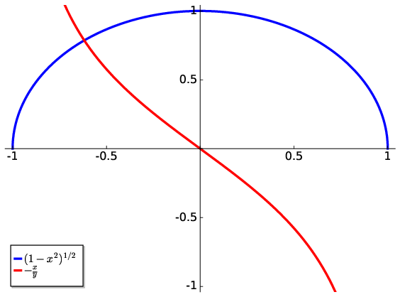
Fig. 3.5 For the positive semi-circle, the derivative is shown in red and tends to infinity as \(|x|\rightarrow1\).

3.4. Logarithmic differentiation

A useful application of implicit differentiation is for functions, \(f(x)\), where \(x\) is an exponent. For example

\[ y=a^x \]

First take the natural logarithm

\[ \ln y=\ln a^x=x \ln a \]

Differentiate both side with respect to \(x\)

\[ \frac{d\ln y}{dx}=\frac{d}{dx}x \ln a \]

Using the chain rule on the left hand side and standard differentiation on the right hand side

\[ \frac{d\ln y}{dy}\frac{dy}{dx}= \ln a \]

Finally using the standard form for the derivative of the natural logarithm

\[ \frac{1}{y}\frac{dy}{dx}= \ln a \]

Rearranging

\[ \frac{dy}{dx}= y\ln a \]

Finally substituting \(y=a^x\) on the right hand side, we obtain an explicit expression for the derivative

\[ \frac{dy}{dx}= a^x\ln a \]