2. Trigonometric and Hyperbolic Functions #

2.1. Trigonometric functions #

Trigonometry functions associate the sides of a right angled triangle to it’s angles. The three basic trigonometry functions are:

  • cosine: ratio of adjacent to hypotenuse

(2.1)#\[ \frac{y}{r}=\cos\theta \]
  • sine: ratio of opposite to hypotenuse

(2.2)#\[ \frac{x}{r}=\sin\theta \]
  • tan: ratio of opposite to adjacent

(2.3)#\[ \frac{x}{y}=\tan\theta=\frac{\sin\theta}{\cos\theta} \]

Since the input angle can be 0-360\(^{\circ}\), these trig functions are typically defined using a circle. If the radius of the circle, i.e the hypotenuse, is set to 1 the sine and cosine ratios reduce to opposite and adjacent respectively. As the angle increases the values of these ratios change and repeat periodically for each cycle around the circle. Due to their periodic nature, trigonometric functions are used frequently in physics to describe oscillating phenomena.

_images/Sin-cos-define.png

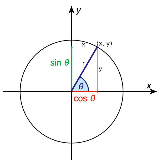
Fig. 2.1 Trigonometric functions relate the ratio of two sides to an angle of a triangle.#

_images/SinCos.png

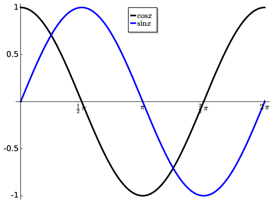
Fig. 2.2 Cosine and sine functions are shown for a single cycle for \(x=0\rightarrow2\pi\). Notice that the functions are identical but differ in phase by \(\pi/2\).#

_images/Tan.png

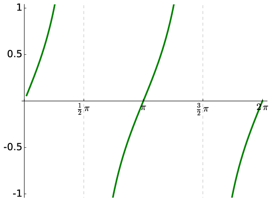
Fig. 2.3 The \(y=\tan x\) function shown for a single cycle for \(x=0\rightarrow2\pi\). Notice the asymptotes at odd multiples of \(\pi/2\) .#

The other three possible ratios should also be noted:

(2.4)#\[\begin{split} \begin{aligned} \mathrm{cosec}\,\theta & =\frac{r}{y}=\frac{1}{\sin\theta}\\ \sec\theta & =\frac{r}{x}=\frac{1}{\cos\theta}\\ \cot\theta & =\frac{x}{y}=\frac{1}{\tan\theta}\end{aligned} \end{split}\]

2.2. Trigonometric identities #

There are many standard identities which can be useful in solving analytical problems in physics. Memory of these is of course not required but you should be aware of their existence or even better practice proving them!

The first set relate the squares of the functions and can be proven via Pythagoras’s Theorem:

\[\begin{split}\begin{aligned} \cos^{2}\theta+\sin^{2}\theta=1\\ 1+\tan^{2}\theta=\sec^{2}\theta\\ \cot^{2}\theta+1=\mathrm{cosec}^{2}\,\theta\end{aligned}\end{split}\]

The double angle formula are:

\[\begin{split}\begin{aligned} {\rm sin}\;2\theta&={\rm sin}\;(\theta+\theta)={\rm sin}\;\theta\;{\rm cos}\;\theta+{\rm cos}\;\theta\;{\rm sin}\;\theta=2{\rm sin}\;\theta{\rm \,cos}\;\theta\\ {\rm cos}\;2\theta&={\rm cos}\;(\theta+\theta)={\rm cos}\;\theta\;{\rm cos}\;\theta-{\rm sin}\;\theta\;{\rm sin}\;\theta={\rm cos}^{2}\;\theta-{\rm sin}^{2}\;\theta\end{aligned} \end{split}\]

The sum formula are:

\[\begin{split} \begin{aligned} {\rm sin}\;A-{\rm sin}\;B & =2{\rm cos}\;(\frac{A+B}{2}){\rm sin}\;(\frac{A-B}{2})\\ {\rm sin}\;(A\pm B)= & {\rm sin}\;A\;{\rm cos}\;B\pm{\rm cos}\;A\;{\rm sin}\;B\\ {\rm cos}\;(A\pm B)= & {\rm cos}\;A\;{\rm cos}\;B\mp{\rm sin}\;A\;{\rm sin}\;B\\ {\rm sin}\;A+{\rm sin}\;B= & 2{\rm sin}\;(\frac{A+B}{2}){\rm cos}\;(\frac{A-B}{2})\\ {\rm sin}\;A-{\rm sin}\;B= & 2{\rm cos}\;(\frac{A+B}{2}){\rm sin}\;(\frac{A-B}{2})\\ {\rm cos}\;A+{\rm cos}\;B= & 2{\rm cos}\;(\frac{A+B}{2}){\rm cos}\;(\frac{A-B}{2})\\ {\rm cos}\;A-{\rm cos}\;B= & -2{\rm sin}\;(\frac{A+B}{2}){\rm sin}\;(\frac{A-B}{2})\\ 2{\rm sin}\;A\;{\rm cos}\;B= & {\rm sin}\;(A+B)-{\rm sin}\;(A-B)\\ 2{\rm sin}\;A\;{\rm sin}\;B= & {\rm cos}\;(A+B)-{\rm cos}\;(A-B)\\ 2{\rm cos}\;A\;{\rm cos}\;B= & {\rm cos}\;(A+B)+{\rm cos}\;(A-B)\\ {\rm tan}\;(A+B)= & \frac{{\rm tan}\;A+{\rm tan}\;B}{1+{\rm tan}\;A\;{\rm tan}\;B} \end{aligned} \end{split}\]

Finally there is the Cosine Rule:

\[c^{2}=a^{2}+b^{2}-2ab\cos C\]

the Sine rule:

\[\frac{\sin A}{a}=\frac{\sin B}{b}=\frac{\sin C}{c}\]

and the area of a triangle:

\[\frac{1}{2}ab\sin C=\frac{1}{2}bc\sin A=\frac{1}{2}ac\sin B\]

2.3. Hyperbolic Functions #

Whereas the standard trigonometric functions are based on circles (\(x^{2}+y^{2}=r^{2}\)), hyperbolic trigonometric functions are based on hyperbola (\(x^{2}-y^{2}=1\)) as shown in Fig. Fig. 2.4. The geometry defined by hyperbolic functions have numerous applications in physics.

_images/UnitHyperbola.png

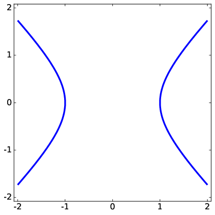
Fig. 2.4 The hyperbola defined by the equation \(x^{2}-y^{2}=1\).#

_images/cosh_sinh.png

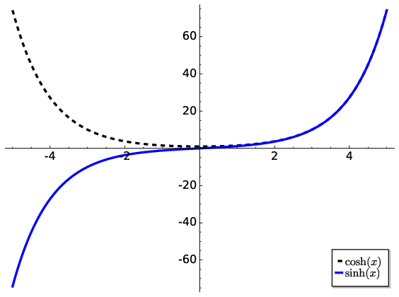
Fig. 2.5 The main hyperbolic functions are shown for \(\sinh x\) and \(\cosh x\)#

_images/tanh.png

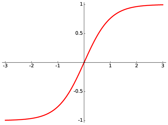
Fig. 2.6 The main hyperbolic functions are shown for \(\tanh x\)#

The functions themselves are combinations of exponential \(e^{x}\) curves and define hyperbolic versions of the trigonometric sine, cosine etc.:

\[\begin{split} \begin{aligned} \sinh x & =\frac{1}{2}\left(e^{x}-e^{-x}\right)\\ \cosh x & =\frac{1}{2}\left(e^{x}+e^{-x}\right)\\ \tanh x & =\frac{\sinh x}{\cosh x}=\frac{\mathrm{e}^{2x}-1}{\mathrm{e}^{2x}+1}\end{aligned} \end{split}\]

The graphs of these functions are shown in Fig. Fig. 2.5 and Fig. Fig. 2.6. There are also corresponding reciprocals:

\[\DeclareMathOperator{\sech}{sech} \sech x = 1/\cosh x\]
\[\DeclareMathOperator{\cosech}{cosech} \cosech x =1/\sinh x \]
\[\DeclareMathOperator{\coth}{coth} \coth x = 1/\tanh x\]