7. Integration

7.1. Indefinite Integrals and Signed Area

Integration is the opposite process to differentiation, and is used to calculate the area under a curve. However in this unit you will discover that integration is a much more powerful tool than simply working out areas, and you will learn methods of integration that are used time and again throughout your degree.

7.1.1. Common Integrals

There are some common integrals with which you should already be faniliar. The following list are ones that you should be able to recall.

\[\begin{split}\begin{aligned} f\left(x\right) & & F\left(x\right)=\int f\left(x\right)dx\\ a\:\mathrm{(constant)} & & ax+c\:\left(\mathrm{c\,is\,constant}\right)\\ x^{n} & & \frac{x^{n+1}}{n+1}+c\\ \frac{1}{x} & & \ln\left|x\right|+c\\ e^{ax} & & \frac{1}{a}e^{ax}+c\\ \cos\left(x\right) & & \sin\left(x\right)+c\\ \sin\left(x\right) & & -\cos\left(x\right)+c\\ \cos\left(ax\right) & & \frac{1}{a}\sin\left(ax\right)+c\\ \sin\left(ax\right) & & -\frac{1}{a}\cos\left(ax\right)+c\end{aligned}\end{split}\]

Note that the constant of integration \(c\) must be included when dealing with indefinite integrals (that is, those that do not have limits specified).

7.1.2. Significance of the areas bounded by the curve.

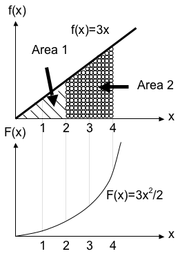
The area between a curve and the x-axis is equal to the integral of the function; for a definite integral we specify limits and consider the signed area under the curve between these limits.

The diagram below shows the function \(f\left(x\right)=3x\) and how the integral \(F\left(x\right)\) gives the area under the function.

7.1.3. Negative area

The convention is that a positive area lies above the x-axis (i.e. \(y > 0\)) whereas a negative area lies below it (i.e. \(y < 0\)).

7.2. Definite integrals

7.2.1. Integration from First Principles

If we take a general function \(f\left(x\right)\) as shown in Fig. 7.1, the area below the curve between limits \(a\) and \(b\) has been divided up into \(N\) slices each with width \(\delta x\) and approximate height \(f\left(x\right)\) - note that this is an approximation but becomes more precise as \(\delta x\) becomes very small.

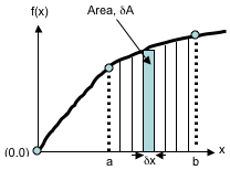
Fig. 7.1 Integration from first principles

In fact, knowing the limits and the number of slices allows us to define the width of a single slice as \(\delta x=\dfrac{\left(b-a\right)}{N}\) and thus we can see that larger N gives us smaller slice width. Each slice has an area \(\delta A\left(x\right)\) and so the total area under the curve is the sum of all slice areas given by

\[ A=\sum_{x=a}^{x=b}\delta A \]

but for small slice width the area is approximately a rectangle with area \(\delta A=f\left(x\right)\delta x\). From this we can see that

\[ \frac{\delta A}{\delta x} = f(x) \]

so that in the limit of \(\delta x \to 0\),

\[\lim_{\delta x \to 0} \frac{\delta A}{\delta x} =\frac{dA}{dx}= f(x)\]

so that we see that the function \(A\) when differentiated gives \(f(x)\); i.e., it is the anti-differential of \(f(x)\). The total area is given by

\[A=\sum_{x=a}^{x=b}f\left(x\right)\delta x\]

If we now decrease the size of \(\delta x\) until it is infinitely small we obtain the final integral form

\[A=\lim_{\delta x\rightarrow0}\sum_{x=a}^{x=b}f\left(x\right)\delta x=\int_{a}^{b}f\left(x\right)dx\]

7.2.2. Improper Integrals

Improper integrals are those in which either the integral has an infinite range (i.e. one or both limits are infinite) or the integrand itself can become infinite for some value of x within the range over which the integral is evaluated.

When dealing with improper integrals, first substitute the limit that is infinity by R then evaluate the integral as normal. Once the integral has been calculated, substitute back to determine the solution given the behaviour of the functions at infinity. We will consider an example to highlight this.

Evaluate

\[\begin{split}\begin{aligned} \int_{0}^{\infty}e^{-2x}dx & = & \lim_{R \to \infty} \int_{0}^{R}e^{-2x}dx \\ & = & \lim_{R \to \infty} \left[-\frac{1}{2}e^{-2x}\right]_{0}^{R}\\ & = & \lim_{R \to \infty} -\frac{1}{2}e^{-2R}-\left(-\frac{1}{2}\right)\\ & = & \lim_{R \to \infty} \frac{1}{2}\left(1-e^{-2R}\right)\\ & = & \frac{1}{2}\left(1-e^{-\infty}\right)\\ & = & \frac{1}{2}\end{aligned} \end{split}\]

which requires knowledge of how the exponential function behaves at the limit of \(-\infty\).

7.2.3. Symmetric Integrals

An even function is defined as \(f\left(x\right)=f\left(-x\right)\) and odd functions defined by \(f\left(x\right)=-f\left(-x\right)\). Fig. 7.2 and Fig. 7.3 shows two examples: the left diagram shows the even function \(f\left(x\right)=x^{4}-x^{2}+3\) and the right is the odd function \(f\left(x\right)=x^{3}-x\).

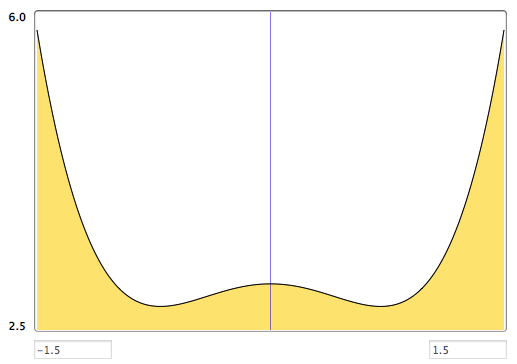
Fig. 7.2 First example of symmetric functions. This is the even function \(f\left(x\right)=x^{4}-x^{2}+3\). Yellow regions are the areas under the curve between symmetric limits.

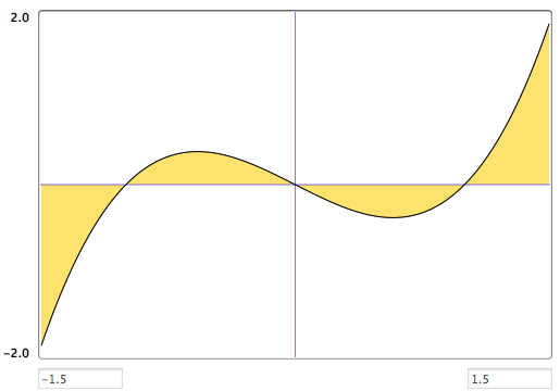
Fig. 7.3 Second example of symmetric functions. This is the odd function \(f\left(x\right)=x^{3}-x\). Yellow regions are the areas under the curve between symmetric limits.

The behaviour of such functions is useful when the limits of the integral are symmetric about \(x = 0\). For example, for even functions the shaded area to the left of the y axis (that is, for negative values of x) is equal to that on the right of the y axis as long as the limits are symmetric about \(x=0\). In integral form this is written as

\[\int_{-a}^{0}f\left(x\right)=\int_{0}^{a}f\left(x\right)\]

and so it follows that

\[\int_{-a}^{a}f\left(x\right)=\int_{-a}^{0}f\left(x\right)+\int_{0}^{a}f\left(x\right)=2\int_{0}^{a}f\left(x\right)\]

for any even function.

The shaded area under the odd function curve is equal in size for \(x<0\) and \(x>0\), but the difference here is in sign - any positive area on the left side of the y axis has an equal but negative counterpart on the right side, and vice versa. This tells us that

\[\int_{-a}^{0}f\left(x\right)=-\int_{0}^{a}f\left(x\right)\]

and therefore

\[\int_{-a}^{a}f\left(x\right)=0\]

for any odd function.

7.3. Methods of integration

7.3.1. Substitution

7.3.1.1. Integrals of the form \(\displaystyle{\int}f\small(ax+b\small)\,\mathrm{d}x\)

For such functions, for example \(f(x)=\left(x-5\right)^5\) or \(f(x) = \sin\left(3x+1\right)\), we utilise the fact that the integrals of functions such as \(x^3\) and \(\sin(x)\) are standard, so we use a substitution to transform the original function into a simpler one.\

Two steps are required: identify the appropriate substitution, which is usually the term inside the brackets, and calculate \(\dfrac{\mathrm{d}u}{\mathrm{d}x}\) to find any factors required to substitute \(\mathrm{d}u\) for \(\mathrm{d}x\). For example:

\[\begin{split}\begin{aligned} y &= \int\sin\left(3x+1\right)\,\mathrm{d}x\\ \text{Let } u&= 3x+1\\ \dfrac{\mathrm{d}u}{\mathrm{d}x} &= 3 \quad \text{or } \mathrm{d}x = \dfrac{\mathrm{d}u}{3}\\ \therefore y &= \int \dfrac{\sin(u)}{3}\,\mathrm{d}u\\ &= -\dfrac{\cos(u)}{3} +c = -\dfrac{\cos(3x+1)}{3} + c\end{aligned}\end{split}\]

7.3.1.2. Integrals of the form \(\displaystyle{\int}f\left(g(x)\right)\,g'(x)\,\mathrm{d}x\)

This method can be used when your integrand contains both a function (sometimes within another function) and its derivative. The difficulty with this method is correctly identifying the appropriate substitution. Once the correct substitution has been identified you must substitute for \(g(x)\), \(g'(x)\) and \(\mathrm{d}x\).

\[\begin{split}\begin{aligned} y&=\int\sin x \cos x \,\mathrm{d}x\\ \text{Let }u&= \sin x\\ \dfrac{\mathrm{d}u}{\mathrm{d}x} &= \cos x \quad \text{or } \mathrm{d}u = \cos x\, \mathrm{d}x\\ \therefore y&= \int u \, \mathrm{d}u\\ &= \dfrac{u^2}{2} +c = \dfrac{\sin^2 x}{2} + c\end{aligned}\end{split}\]

In the next example we will see how the substitution function can be within another function.

\[\begin{split}\begin{aligned} y&= \int 6x\cos x^2 \,\mathrm{d}x\\ \text{Let }u&=x^2\\ \dfrac{\mathrm{d}u}{\mathrm{d}x} &= 2x \quad \text{or } \mathrm{d}u = 2x\, \mathrm{d}x\end{aligned}\end{split}\]

We need to multiply both sides by \(3\) so that we have the term \(6x\,\mathrm{d}x\) present in the original function. Thus

\[\begin{split}\begin{aligned} \therefore y&= 3\int\cos(u) \, \mathrm{d}u\\ &= 3\sin(u) + c = 3\sin(x^2)+c\end{aligned}\end{split}\]

7.3.1.3. Using trigonometric and hyperbolic identities

As with other substitution methods this one requires you to identify the appropriate function to substitute. However some of these require you to already know, from experience, what substitution to use.[1] Identities such as the following will be useful:

\[\begin{split}\begin{aligned} \sin^2 x +\cos^2 x &= 1\\ 1+\tan^{2}\left(x\right)&=\sec^{2}\left(x\right) \\ 1-\tanh^{2}\left(x\right)&=\mathrm{sech^{2}}\left(x\right) \\ 1+\sinh^{2}\left(x\right)&=\cosh^{2}\left(x\right) \end{aligned}\end{split}\]

As will knowledge of the following standard differentials:

\[\begin{split}\begin{aligned} \frac{d}{dx}\tan\left(x\right)&=\sec^{2}\left(x\right)\\ \frac{d}{dx}\tanh\left(x\right)&=\mathrm{sech^{2}\mathit{\left(x\right)}}\\ \frac{d}{dx}\sinh\left(x\right)&=\cosh\left(x\right)\\ \frac{d}{dx}\cosh\left(x\right)&=\sinh\left(x\right)\end{aligned}\end{split}\]

Consider the integral \(\displaystyle{\int}\dfrac{1}{\left(1+x^2\right)}\,\mathrm{d}x\). We will make use of the property \(1+\tan^2 x = \sec^2 x\)

\[\begin{split}\begin{aligned} \text{Let } x &= \tan u\\ \dfrac{\mathrm{d}x}{\mathrm{d}u} &= \sec^2 u \qquad \text{so }\mathrm{d}x = \sec^2 u \mathrm{d}u\\ \therefore \int\dfrac{1}{1+x^2}\,\mathrm{d}x &= \int\dfrac{1}{1+\tan^2 u}\sec^2 u \,\mathrm{d}u\\ &= \int\dfrac{\sec^2 u}{\sec^2 u}\,\mathrm{d}u = \int \, \mathrm{d}u\\ &= u + c \\ & = \tan^{-1}x+ c\end{aligned} \end{split}\]

There isn’t really a shortcut for this method - it comes with practice and familiarity with identities.

7.3.1.4. Definite integrals and substitution

When using substitution with definite integrals, you need to change the limits of integration since these are usually different for the new variable. For example

\[\begin{split}\begin{aligned} I & = & \int_{1}^{2}\left(3x-2\right)^{3}dx\\ & = & \int_{u_{1}}^{u_{2}}\frac{u^{3}}{3}du\:\mathrm{\:where\:}\:u=3x-2\end{aligned} \end{split}\]

We need to calculate the new limits \(u_{1}\) and \(u_{2}\) using the substitution solved at each of the original limits, or

\[\begin{split}\begin{aligned} u_{1} & = & u\left(x=1\right)=\left(3\times1\right)-2=1\\ u_{2} & = & u\left(x=2\right)=\left(3\times2\right)-2=4\end{aligned}\end{split}\]

and so the integral is

\[\begin{split}\begin{aligned} I & = & \int_{1}^{4}\frac{u^{3}}{3}du\\ & = & \left[\frac{u^{4}}{12}\right]_{1}^{4}\\ & = & \frac{255}{12}\end{aligned} \end{split}\]

An alternative method that avoids changing the limits is by substituting back in and using the original limits

\[\begin{split}\begin{aligned} I & = & \int_{u_{1}}^{u_{2}}\frac{u^{3}}{3}du\\ & = & \left[\frac{u^{4}}{12}\right]_{u_{1}}^{u_{2}}\\ & = & \left[\frac{\left(3x-2\right)^{4}}{12}\right]_{1}^{2}\\ & = & \frac{256}{12}-\frac{1}{12}=\frac{255}{12}\end{aligned} \end{split}\]

---

[1]

This emphasises the need for practice, so that you recognise these substitutions when they arise.