6. Taylor Series, L’Hopital’s rule and approximation errors

6.1. Taylor series centred at \(x=c\)

There are cases where a function cannot be defined as a Taylor series centered at zero. A good example is when there are no derivatives at \(x=0\) such as for \(\ln(x)\). The area of interest may not be near zero either. In such cases we can define a Taylor series approximation of the function centered at some point \(c\) using the more general form:

\[\begin{split}\begin{aligned} f(x) & =\sum_{n=0}^{\infty}\frac{f^{(n)}(c)}{n!}(x-c)^{n}\\ & =f(c)+f^{(1)}(c)(x-c)+\frac{f^{(2)}(c)}{2}(x-c)^{2}+\cdots\end{aligned}\end{split}\]

You will also see this form written where the difference \(x-c=u\) so \(x=c+u\):

\[\begin{split}\begin{aligned} f(u+c) & =\sum_{n=0}^{\infty}\frac{f^{(n)}(c)}{n!}u^{n}\\ & =f(a)+hf^{(1)}(c)+\frac{h^{2}f^{(2)}(c)}{2}+\cdots\end{aligned}\end{split}\]

6.2. Indeterminate values: l’Hospital’s Rule

An indeterminate value is often in the form such as \({\displaystyle {\frac{0}{0}},~{\frac{\infty}{\infty}}}\) and \({\displaystyle 0\times\infty,~1^{\infty},~\infty-\infty,~0^{0}{\text{ and }}\infty^{0}.}\) These are distinct from similar looking expressions such as \(0/\infty\) = 0. Indeterminate values typically occur when evaluating functions at some limit especially when comprised of a numerator and denominator. For example, the function:

\[f(x)=\frac{\sin(x)}{x}\]

is undefined at \(x=0\) since \(f(0)=0/0\). However, the limit as \(x\rightarrow0\) does exist and can be determined by evaluating the derivatives of the numerator and denominator. To do so we can approximate the numerator and denominator as two Taylor series:

\[\frac{f(x)}{g(x)}=\frac{f(0)+f^{(1)}(0)x+f^{(2)}(0)x^{2}/2+\cdots}{g(0)+g^{(1)}(0)x+g^{(2)}(0)x^{2}/2+\cdots}\]

and since \(f(0)=g(0)=0\):

\[\frac{f(x)}{g(x)}=\frac{f^{(1)}(0)x+f^{(2)}(0)x^{2}/2+\cdots}{g^{(1)}(0)x+g^{(2)}(0)x^{2}/2+\cdots}=\frac{f^{(1)}(0)+f^{(2)}(0)x/2+\cdots}{g^{(1)}(0)+g^{(2)}(0)x/2+\cdots}\]

and taking the limit:

\[\lim_{x\to0}\frac{f(x)}{g(x)}=\frac{f^{(1)}(0)}{g^{(1)}(0)}\]

which can be generalised for any limit \(a\):

\[\lim_{x\to a}\frac{f(x)}{g(x)}=\frac{f^{(1)}(a)}{g^{(1)}(a)}\]

Evaluating the quotient of the derivatives may then provide a real or indeed an infinite value for the limit. If not than the next higher derivatives are used and so on until the limit can be evaluated. This method is typically referred to as l’Hospital’s Rule (pronounced as lopital’s Rule). In the case of

\[\lim_{x\to0}\frac{\sin(x)}{x}\]

we can evaluate the first derivatives:

\[\lim_{x\to0}\frac{\cos(x)}{1}=\frac{1}{1}=1\]

which is a real determinate value.

An example where the second derivatives are needed is:

\[\begin{split}\begin{aligned} \lim_{x\to0}\frac{1-\cos(x)}{x^{2}}=\lim_{x\to0}\frac{\sin(x)}{2x} & =\frac{0}{0}\\ & =\lim_{x\to0}\frac{\cos(x)}{2}=\frac{1}{2}\end{aligned} \end{split}\]

Infinity is also a possible outcome of applying such limits. For example:

\[\lim_{x\to0}\frac{e^{x}-1}{x^{3}}=\lim_{x\to0}\frac{e^{x}}{3x^{2}}=\frac{1}{0}=\infty\]

Such functions, which originally appeared indeterminate, can thus be analysed to yield real or infinite values. These examples are visualised in Fig. 6.1.

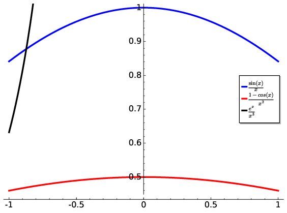
Fig. 6.1 Example of functions which have indeterminate values at \(x=0\). Using l’Hospital’s Rule we can show that the example functions comprised of sine and cosine terms produce a finite value at \(x=0\) whereas the exponential function does to infinity.

6.3. Evaluating errors of approximations

As mentioned at the beginning of this section, it is important to be aware of the imperfections of approximations. In many cases, we can be content in approximating some function to within some acceptable accuracy. In other cases, the approximation may be not justified and hence be just wrong. Developing methods to evaluate accuracy is indeed useful especially if we are to defend applications in physical theories.

When computing approximations it is useful to define key concepts:

• Accuracy: how close our approximation is to the actual value

• Precision: how many digits we have in our approximation.

We can assess these two quantities by computing the following errors:

• Absolute Error

• Relative Error

Of course, since we do not typically know the exact value of the function, we can only estimate the errors. But this is still useful. In some cases, we may know the exact value of \(f(x)\) but choose to use an approximation for faster calculations. We can then test to prove if we are achieving some desired accuracy. Numerically, we can just calculate an approximation and compare it to the real value. For example, computing \(\cos(x)\) for \(n=10\) requires just the first 6 terms of the series centred at zero:

\[ \cos x=1-\frac{x^{2}}{2!}+\frac{x^{4}}{4!}-\frac{x^{6}}{6!}+\frac{x^{8}}{8!}-\frac{x^{10}}{10!}\ldots \]

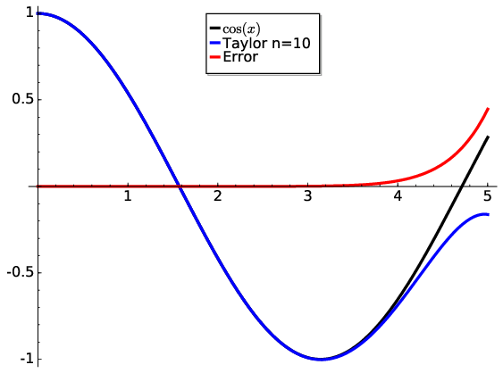
Fig. 6.2 A Taylor approximation of a cosine function using a 10 degree polynomial. While centred at zero, the Taylor series is relatively accurate up until \(x\approx4\). This accuracy is also shown by the error curve.

We can see via Fig. 6.2 that the approximation is good until near \(x=4\). Afterwards the series diverges from the exact solution. By \(x=5\) the absolute error is approaching 0.3. For such trigonometric functions, an infinite number of terms are needed. However, in most cases we are only interested in a certain region of the domain \(x\) so an approximation suffices.

Analytically, we can estimate the absolute error or remainder for some \(n\)-degree Taylor expansion \(T_{n}(x)\):

\[R_{n}=\left|f(x)-T_{n}(x)\right|\]

Since the Taylor approximation becomes more accurate as more terms are included, the \(T_{n+1}(x)\) polynomial must be more accurate than \(T_{n}(x)\):

\[T_{n+1}(x)=T_{n}(x)+f^{n+1}(a)\frac{(x-a)^{n+1}}{(n+1)!}\]

The error in \(T_{n}(x)\) then can be no larger than the last term:

\[R_{n}\leq\max\big(f^{(n+1)}(a)\big)\frac{(x-a)^{n+1}}{(n+1)!}\]

What does this mean? The expression provides an upper limit of the absolute error at some value of \(x\) for a series centred at \(a\). Since we are using a \(\cos x\) example, the \(|f^{(n+1)}|\) derivative will never be greater than one i.e. each successive derivative will \(\sin\) or \(\cos\). Therefore here \(\max\big(f^{(n+1)}(a)\big)=1\) and since we are centred at zero, \(a=0\), our analytical estimate will be

\[R_{n}\leq\frac{x^{n+1}}{(n+1)!}\]

For small \(x\), this predicts a very small error approaching zero i.e. the series converges to the exact value. For example at \(x=1\) and using \(n=10\) the remainder is \(R_{n}=\leq\frac{2^{11}}{11!}=0.00005\). Hence our approximation is accurate to 4 decimal places with \(n=10\). We can then proceed along \(x\) until our estimate becomes too large for comfort such as by \(x=5\) where it is much larger than \(f(x)\) with \(R_{n}=1.22\) as shown in Fig. 6.3.

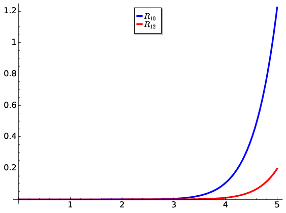
Fig. 6.3 Adding more terms to the Taylor series reduces the error at the expense of increased computations. Here we visualise the remainder function, \(R_{n}\), for \(n=10\) and \(n=12\) series approximating the cosine function centred at \(x=0\).