11. Vectors

The material in this topic is also covered in chapter 8 of the textbook Martin and Shaw “Mathematics for Physicists”. In Boas “Mathematical Methods in the Physical Sciences” it is in chapter 3 sections 4 and 5 and in chapter 6 sections 2 and 3.

11.1. Introduction

Vectors are an essential mathematical tool for describing many physical phenomena. They allow us to encode the concept of directionality in a physical quantity. Familiar examples include velocity, which requires both a speed and a direction of travel, and force, which requires a magnitude and direction in which the force is acting. By developing knowledge of the mathematics of vectors you will become familiar with some powerful tools that simplify manipulations and calculations that are of relevance to physics ranging from classical mechanics and electromagnetism to relativity.

In this introductory course we will only consider 2 and 3 dimensional Cartesian space, but the concepts can be extended and applied to other spaces, for example, 4 dimensional space-time coordinate systems for special relativity and curved spaces for general relativity.

11.2. Definitions

11.2.1. Vectors in Cartesian coordinates

A vector is a list of numbers that together define an arrow in space i.e. specify its length and its direction. For example for a velocity, \(\vec{v}\), its length is the speed and its direction is the direction of motion. Vectors can be written in several different ways. For example a row vector is written as a list of numbers in a row:

\[\vec{v}=(\begin{array}{ccc}a&b&c\end{array})\]

where \(a\), \(b\) and \(c\) are numbers. Sometimes commas are used to separate the numbers in the list of a row vector i.e.

\[\vec{v}=(a,b,c)\]

We call these the numbers \(a\), \(b\) and \(c\) the components or elements of the vector. A column vector lists the elements in a column i.e.

\[\begin{split}\vec{v}=\left(\begin{array}{c}a\\b\\c\end{array}\right)\end{split}\]

Often in typed documents and textbooks bold font is used to indicate that a quantity is a vector as I have used here for the vector \(\vec{v}\). However, in handwriting and on a blackboard it is not easy to write in bold font and therefore other conventions are used such as an arrow above the letter or a line underneath it;

\[\vec{v}=\vec{v}=\underline{v}\]

Each of these notations mean the same thing i.e. that this quantity is a vector not a scalar which would be written as \(v\). A scalar is a single number such as speed whereas velocity is a vector so needs several components. To specify a vector in space we need one component for each dimension e.g. for 3D space we need 3 components as in my example \(\vec{v}\) above. To describe space we use a coordinate system. Here we will use the coordinate system you are most familiar with, the Cartesian coordinate system i.e. \(x\), \(y\), \(z\) axes. Each element gives the component in that direction. In our example \(\vec{v}\) defined above \(a\) is the \(x\) component, \(b\) is the \(y\) component and \(c\) is the \(z\) component. To draw the arrow described by the vector \(\vec{v}\) on a graph we simply plot the coordinates \((a,b,c)\) and draw an arrow from the origin to this point, as done in figure Fig. 11.1 for a vector \(\vec{v}=(\:a\:\:\:b\:)\) in 2D (two dimensional) Cartesian \(x\)-\(y\) space.

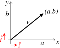
Fig. 11.1 The vector \(\vec{v}=(\:a\:\:\:b\:)\) is plotted as a large black arrow on a graph of 2D Cartesian space with axes x and y. The basis vectors are indicated as small red arrows.

11.2.2. Basis vectors

To express a vector in space, we must first define a coordinate system. We do this be specifying the axes e.g. the \(x\), \(y\), \(z\)-axes for the Cartesian coordinate system. We can define these axes using basis vectors. These are vectors of length one unit in the directions we want the axes to be in. A vector of length one is called a unit vector and is usually denoted by a hat on top e.g. \(\hat{\vec{x}}\). The basis vector in the \(x\) direction is sometimes called \(\hat{\vec{i}}\). The \(x\) and \(y\) basis vectors are indicated on Fig. 11.1.

Since the 3 basis vectors in the Cartesian coordinate system are mutually perpendicular we can write any point in space as a combination of the basis vectors. There are several notations used for the basis vectors in the Cartesian coordinate system and it is worth remembering them all since different lecturers/books will use them interchangably. Let us express our velocity vector from the previous section in terms of the basis vectors;

\[\begin{split}\begin{aligned} \vec{v} &= a\hat{\vec{i}} + b\hat{\vec{j}} + c\hat{\vec{k}}\\ &= a\hat{\vec{x}} + b\hat{\vec{y}} + c\hat{\vec{z}}\\ &=a\hat{\vec{e_x}} + b\hat{\vec{e_y}} + c\hat{\vec{e_z}}\\ &=a\hat{\vec{e_1}} + b\hat{\vec{e_2}} + c\hat{\vec{e_3}} \end{aligned}\end{split}\]

The component \(a\) gives the speed in the \(x\) direction and the component \(b\) the speed in the \(y\) direction etc. To remind ourselves of this meaning of the components it can be helpful to write them as \(a=v_x\), \(b=v_y\) and \(c=v_z\) i.e.

\[\vec{v} = v_x\hat{\vec{i}} + v_y\hat{\vec{j}} + v_z\hat{\vec{k}}\]

where the subscripts indicate the relevant component.

11.2.3. Magnitude/Modulus

The magnitude, also known as the modulus, of a vector is the length of the arrow specified by the vector. By Pythagoras’ theorem this length is given by

\[v=\left|\vec{v}\right|=\sqrt{v_{x}^2 + v_{y}^2 + v_{z}^2}.\]

If the vector represents velocity, its magnitude is the speed. Note that the letter without its bold font or arrow indicating the vector is often used to denote the magnitude of the vector i.e. the speed is \(v\) and the velocity is \(\vec{v}\). However if this distinction is a bit subtle it is safer to use the modulus signs \(|\vec{v}|\).

Note that this definition of the magnitude is true for any vector, not just the velocity. For example let us define a general vector \(\vec{a}\) as

\[\vec{a} = a_x\hat{\vec{i}} + a_y\hat{\vec{j}} + a_z\hat{\vec{k}}\]

the the magnitude of \(\vec{a}\) is

\[a=\left|\vec{a}\right|=\sqrt{a_{x}^2 + a_{y}^2 + a_{z}^2}.\]

11.2.4. Unit vectors

We’re already met unit vectors in the context of basis vectors but we can also define a unit vector for any vector as the vector of magnitude one in the direction of the vector of interest. For our general vector \(\vec{a}\) we can define its unit vector as

\[\hat{\vec{a}}=\frac{a_{x}}{a} \hat{\vec{i}} + \frac{a_{y}}{a} \hat{\vec{j}} + \frac{a_{z}}{a} \hat{\vec{k}}\]

corresponding to a unit vector in the direction of \(\vec{a}\).

11.3. Manipulating vectors

11.3.1. Addition and subtraction of vectors

In physics we often need to add vectors. For example, to find the net force we often need to add forces that are actin in different directions. You know Newton’s second law, \(F=ma\) in scalar form which is valid for one dimensional problems. But in 2D or 3D space force and acceleration are vectors i.e. \(\vec{F}=m\vec{a}\). To find the resulting acceleration of an object subject to several forces, we need to use vector addition of the forces.

Graphically (see Fig. 11.2) we can add vectors using the triangle (or parallelogram) law. To add a vector \(\vec{b}\) to a vector \(\vec{a}\), we displace \(\vec{b}\), without changing its orientation, so that it starts where \(\vec{a}\) ends i.e. place the tail of the arrow representing \(\vec{b}\) at the head of the arrow \(\vec{a}\). Then we draw the line joining the start of \(\vec{a}\) to the end of \(\vec{b}\) (from the tail of \(\vec{a}\) to the head of \(\vec{b}\)) to get the vector representing the addition of \(\vec{a}\) and \(\vec{b}\). This is shown in Fig. 11.2.

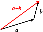
Fig. 11.2 Diagram to show the addition of two vectors. The vectors \(\vec{a}\) and \(\vec{b}\) are plotted as black arrows and their sum \(\vec{a}+\vec{b}\) is the red arrow.

However we don’t actually need to plot vectors to add them. We can find \(\vec{a}+\vec{b}\) algebraically by adding their components i.e.

\[\begin{split}\begin{aligned} \vec{a}+\vec{b}=&a_x\hat{\vec{i}} + a_y\hat{\vec{j}} + b_x\hat{\vec{i}} + b_y\hat{\vec{j}} =(a_x+b_x)\hat{\vec{i}} + (a_y+b_y)\hat{\vec{j}}\\ \vec{a}+\vec{b}=&\left(\begin{array}{c}a_x\\a_y\end{array}\right)+\left(\begin{array}{c}b_x\\b_y\end{array}\right)=\left(\begin{array}{c}a_x+b_x\\a_y+b_y\end{array}\right)\\ \end{aligned}\end{split}\]

where each of the notation examples I have given are equivalent.

Vector addition is commutative, that is adding \(\vec{b}\) to \(\vec{a}\) is the same as adding \(\vec{a}\) to \(\vec{b}\), i.e.

\[\vec{b}+\vec{a}=\vec{a}+\vec{b}.\]

Vector addition is also associative, meaning that if we add three or more vectors, the order in which we do the addition does not matter, i.e.

\[\vec{a}+(\vec{b}+\vec{c})=(\vec{a}+\vec{b})+\vec{c}\]

Vector subtraction, e.g., \(\vec{a}-\vec{b}\), is done by adding the negative of \(\vec{b}\) to \(\vec{a}\). The negative of a vector simply corresponds to reversing its direction so it points the opposite way.

11.3.2. Scalar multiplication

A vector multiplied by a positive scalar, \(k\), has the same direction as the original vector but has a magnitude (length) that is \(k\) times longer which corresponds to multiplying each component by \(k\) i.e.

\[\begin{split}\begin{aligned} k\vec{a}=&k(a_x\hat{\vec{i}} + a_y\hat{\vec{j}}) =ka_x\hat{\vec{i}} + ka_y\hat{\vec{j}}\\ k\vec{a}=&k\left(\begin{array}{c}a_x\\a_y\end{array}\right)=\left(\begin{array}{c}ka_x\\ka_y\end{array}\right)\\ k\vec{a}=&k(a_x,a_y)=(ka_x,ka_y) \end{aligned}\end{split}\]

This follows on directly from the rules of addition discussed in the previous section e.g. \(\vec{a}+\vec{a}+\vec{a}=3\vec{a}\).

If we multiply a vector by a negative scalar, \(-k\), the magnitude again increases by a factor of \(k\) but the direction is reversed.

The multiplication of vectors by scalars obey the following standard rules of multiplication

\[\begin{split}\begin{aligned} k(\vec{a}+\vec{b})=&k\vec{a}+k\vec{b}\\ (p+q)\vec{a}=&p\vec{a}+q\vec{a}\\ p(q\vec{a})=&(pq)\vec{a}=pq\vec{a} \end{aligned}\end{split}\]

where \(k\), \(p\) and \(q\) are scalars.

11.3.3. The dot product

Multiplication of vectors is more complicated than addition or subtraction. There are different kinds of products of two vectors. One, called the scalar product, gives a result which is a scalar. Another type of product, called the vector product, gives a result which is a vector. We will discuss the vector product in section Cross Product. There is a third type of product of two vectors, called the outer product, which results in a matrix. Here we discuss the scalar product which is also called the dot product or inner product.

If \(\vec{a} = a_x\hat{i} + a_y\hat{j} + a_z\hat{k}\) and \(\vec{b} = b_x\hat{i} + b_y\hat{j} + b_z\hat{k}\), then the scalar, or dot, product is given by

(11.1)\[ \vec{a}\cdot\vec{b}=\vec{a}\cdot\vec{b} = a_xb_x + a_yb_y +a_zb_z = ab\cos{\theta} \]

where \(\theta\) is the angle between the two vectors. Note that the result is a scalar, which is why we call it the scalar product. Note also that that to denote this kind of product between vectors we use a dot \(\cdot\) which is why it is also called it the dot product. Note that the dot product between two perpendicular vevctors is zero.

From equation (11.1), we can see that the scalar product is commutative; i.e.,

\[ \underline{a}\cdot\underline{b} = \underline{b}\cdot\underline{a} \]

It is also distributive, meaning that,

\[ \vec{a}\cdot(\vec{b}+\vec{c})=\vec{a}\cdot\vec{b}+\vec{a}\cdot\vec{c} \]

If we multiply a scalar product by a scalar, \(k\), then we have the following equalities,

\[ k(\vec{a}\cdot\vec{b})=(k\vec{a})\cdot\vec{b}=\vec{a}\cdot(k\vec{b}) \]

We can use the scalar product to find the angle between two lines by rearragning equation (11.1) to obtain;

\[ \theta = \cos^{-1}\left(\frac{\vec{a}\cdot\vec{b}}{ab}\right). \]

The special case of finding whether two lines are perpendicular, which corresponds to the scalar product being zero, is particularly useful in physics.

Another very common use of the scalar product in phyics is to find the component of a vector in a particular direction. We often want to know the component of a force in a particular direction. For example it is often useful to resolve forces into perpendicular directions i.e. find the component of a force in each perpendicular direction. In general, if we wish to find the component of \(\vec{a}\) in the direction of \(\vec{b}\), then we take the scalar product of \(\vec{b}\) with the unit vector parallel to \(\vec{b}\); i.e.,

\[ a_b=\vec{a}\cdot\hat{\vec{b}}=a\cos{\theta}. \]

where \(\theta\) is the angle between the vectors \(\vec{a}\) and \(\vec{b}\) and the subscript is used to denote the component in that direction i.e. \(a_b\) is teh component of \(\vec{a}\) in the direction of \(\vec{b}\). This is also known as the projection of \(\vec{a}\) onto \(\vec{b}\). Often the directions we are interested in correspond to the Cartesian axes directions \(\hat{\vec{x}}\), \(\hat{\vec{y}}\), \(\hat{\vec{z}}\). For example the component of a force \(\vec{f}\) along the \(x\) axis would be given by;

\[ f_x=\vec{f}\cdot\hat{\vec{x}}=f\cos{\theta} \]

where \(\theta\) is the angle between the force \(\vec{f}\) and the \(x\)-axis.

11.3.4. The cross product

The cross product, or vector product of two vectors \({\vec{a}}\) and \({\vec{b}}\) is denoted by \(\vec{a}\,\times\,\vec{b}\) is defined as a vector \({\vec{c}}\) which is perpendicular to both \({\vec{a}}\) and \({\vec{b}}\). It has a direction and a magnitude which is equal to the area of the parallelogram that the vectors span. The following formula can be used to define the cross product:

\[\vec{a}\,\times\,\vec{b} = \left|\vec{a}\,\right|\left|\vec{b}\,\right|\sin{\theta} \vec{n}\]

In this equation \(\theta\) is the angle between \(\vec{a}\) and \(\vec{b}\), and n is the unit vector parallel to the plane. See figure Fig. 11.3

The cross product can also be expressed as a three–by–three determinant

\[\begin{split}\begin{aligned} \vec{a}\,\times\,\vec{b} & = & {\left|\begin{array}{ccc}\hat{\vec{i}}&\hat{\vec{j}}&\hat{\vec{k}}\\ a_x&a_y&a_z\\b_x&b_y&b_z\end{array}\right|}\\ &&\\ & = &(a_yb_z - a_zb_y)\,\hat{\vec{i}}- (a_xb_z-a_zb_x)\,\hat{\vec{j}} + (a_xb_y - a_yb_x)\,\hat{\vec{k}} \end{aligned}\end{split}\]

Note that the result of the cross product of two vectors is another vector. This is why it is called the vector product. We denote this type of product using a cross \(\times\) which is why it is also called the cross product.

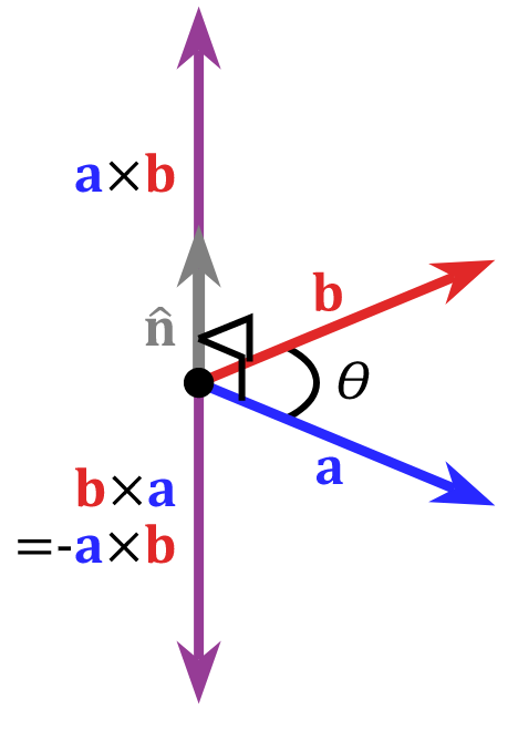
Fig. 11.3 Diagram to show the cross product with of a right-handed coordinate system.

An important feature of the cross product is that it is perpendicular to both of the original vectors.

Note that the cross product is anticommutative meaning it changes sign if the order of the vectors is swapped i.e.

\[ \vec{a}\times\vec{b} = -\vec{b}\times\vec{a} \]

It is distributive i.e.

\[ \vec{a}\times(\vec{b}+\vec{c})=\vec{a}\times\vec{b}+\vec{a}\times\vec{c} \]

Cross products occur in many areas of physics, for example, the force on a particle with charge \(q\) moving with velocity \(\vec{v}\) in a magnetic field \(\vec{B}\) is given by \(\vec{F}=q\vec{v}\times\vec{B}\). The resultant force is perpendicular to both the direction of movement and the magnetic field.

The magnitude of the vector product is given by

(11.2)\[ \left|\vec{a}\,\times\,\vec{b}\,\right| = a\,b\,|\sin{\theta} | \]

Hence the cross product (as well as the dot product) also provides a method for finding the angle between two vectors. Note that the cross product between two parallel vectors is zero.

11.3.5. Triple product

The triple product is the product of three vectors. The scalar triple product results in a scalar whereas the vector triple product results in a vector.

The scalar triple product is given by the dot product between one vector and the cross product of the other two vectors i.e.

\[ \vec{a}\cdot(\vec{b}\times\vec{c}) \]

The triple scalar product can be obtained from the three–by–three determinant of the matrix with the vectors as the rows i.e.

\[\begin{split} \begin{aligned} \vec{a}\cdot(\vec{b}\times\vec{c}) & = & {\left|\begin{array}{ccc} a_x&a_y&a_z\\b_x&b_y&b_z\\c_x&c_y&c_z\end{array}\right|}\\ &&\\ & = &a_x(b_yc_z - b_zc_y)- a_y(b_xc_z-b_zc_x)+ a_z(b_xc_y - b_yc_x) \end{aligned} \end{split}\]

Changing the vector one starts with in a triple scalar product does not change the value as long as the circular order of the vectors is maintained i.e.

\[ \vec{a}\cdot(\vec{b}\times\vec{c})=\vec{b}\cdot(\vec{c}\times\vec{a})=\vec{c}\cdot(\vec{a}\times\vec{b}) \]

Swapping the order of the operations does not change the value i.e.

\[ \vec{a}\cdot(\vec{b}\times\vec{c})=(\vec{a}\times\vec{b})\cdot\vec{c} \]

But swapping the order or any two of the vectors changes the sign of the triple product i.e.

\[\begin{split} \begin{aligned} \vec{a}\cdot(\vec{b}\times\vec{c})=&-\vec{a}\cdot(\vec{c}\times\vec{b})\\ =&-\vec{b}\cdot(\vec{a}\times\vec{c})\\ =&-\vec{c}\cdot(\vec{b}\times\vec{a}) \end{aligned} \end{split}\]

Note that, since the the cross product between parallel vectors is zero and the dot product of perpendicular vectors is zero and the cross product of two vectors is perpendicular to both the original vectors, the triple scalar product is zero if any two of the original vectors are equal i.e.

\[\vec{a}\cdot(\vec{a}\times\vec{b})=\vec{a}\cdot(\vec{b}\times\vec{a})=\vec{a}\cdot(\vec{b}\times\vec{b})=\vec{b}\cdot(\vec{a}\times\vec{a})=0.\]

The vector triple product is the cross product between one vector and the cross product of the other two vectors i.e.

\[\vec{a}\times(\vec{b}\times\vec{c})\]

The vector triple product expansion is given by the following relationship:

\[\vec{a}\times(\vec{b}\times\vec{c})= (\vec{a}\cdot\vec{c})\vec{b} - (\vec{a}\cdot\vec{b})\vec{c}\]

Since the cross product is anticommutative (changes sign when we swap the order) we have;

\[(\vec{a}\times\vec{b})\times\vec{c}=-\vec{c}\times(\vec{a}\times\vec{b})\]

From this we can also find that

\[\vec{a}\times(\vec{b}\times\vec{c})+\vec{b}\times(\vec{c}\times\vec{a})+\vec{c}\times(\vec{a}\times\vec{b})=0\]

and therefore

\[(\vec{a}\times\vec{b})\times\vec{c}=\vec{a}\times(\vec{b}\times\vec{c})-\vec{b}\times(\vec{a}\times\vec{c})\]

11.4. Lines and planes

11.4.1. Equation of a line

In the Cartesian coordinate system, we can describe any straight line by an equation using vectors. The position vector, \(\vec{r}=(x,y,z)\) of any point on the line is given by

(11.3)\[ \vec{r} = \vec{a} + \lambda \vec{c} \]

where \(\lambda\) is a scalar, \(\vec{a}=(a_{x},a_{y},a_{z})\) is the position vector of a point on the line and \(\vec{c}=(c_{x},c_{y},c_{z})\) is a vector parallel to the line (see Fig. 11.4). This form of the equation of a line is called the parametric form.

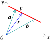
Fig. 11.4 Plot showing the equation of a line using vectors.

Since, a vector has components in each of the directions, the line in equation (11.3) can also be expressed in a symmetric form as;

\[ \frac{x-a_{x}}{c_{x}} = \frac{y-a_{y}}{c_{y}} = \frac{z-a_{z}}{c_{z}} = \lambda \]

Alternatively, if we know the coordinates of two points on a line, \(\vec{a}\) and \(\vec{b}\), then the line can be expressed in parametric form as;

\[ \vec{r} = \vec{a} + \lambda (\vec{b}-\vec{a}) \]

since the difference between the position vectors of two points on the line gives a vector along the line i.e. a vector in the direction of \(\vec{c}\) in equation (11.3). This relationship is a direct consequence of the triangle law of vector addition (see figure Fig. 11.2).

11.4.2. Equation of a plane

We can also use vectors to write down an equation for a plane (see figure Fig. 11.5. The parametric equation of a plane which passes through a point with position vector \(\vec{c}\), and which contains non-parallel vectors \(\vec{a}\) and \(\vec{b}\) is

\[\vec{r} = \vec{c} + \lambda \vec{a} + \mu \vec{b}\]

where \(\lambda\) and \(\mu\) are scalars.

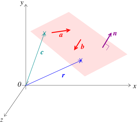
Fig. 11.5 Plot showing the equation of a plane using vectors.

Alternatively, the equation of a plane may also be defined using the scalar and vector product. Since the cross product of two vectors is perpendicular to both vectors, the cross product between two non-parallel vectors that lie in the plane is perpendicular to the plane. A vector perpendicular to a plane is called the vector normal to the plane and often denoted, \(\vec{n}\). So for non-parallel vectors \(\vec{a}\) and \(\vec{b}\) that lie in plane the normal to the plane is given by \(\vec{n}=\vec{a} \times \vec{b}\). The scalar product of any vector that lies in the plane with the normal \(\vec{n}\) must be zero since the scalar product of perpendicular vectors is zero. The vector between any two points in the plane is parallel to the plane and therefore perpendicular to the normal vector \(\vec{n}\). Therefore the vector between some general point on the plane with position vector \(\vec{r}\) and the point on the plane with position vector \(\vec{c}\) must lie in the plane. This vector can be written as \((\vec{r} - \vec{c})\) and since it lies in the plane it must be perpendicular to the normal vector \(\vec{n}\). Therefore the scalar product between \((\vec{r} - \vec{c})\) and \(\vec{n}\) must be zero i.e.,

(11.4)\[\begin{split} \begin{aligned} (\vec{r} - \vec{c}) \cdot \vec{n} &= 0\nonumber\\ \vec{r}\cdot\vec{n}& = \vec{c}\cdot\vec{n} \end{aligned} \end{split}\]

The perpendicular distance from the plane to the origin, \(d\), is given by the projection of the position vector of any point in the plane onto the unit normal, \(\hat{\vec{n}}=\vec{n}/|\vec{n}|\), i.e.

\[ d=\vec{c}\cdot\hat{\vec{n}}. \]

This enables us to write the equation of a plane from (11.4) in the more compact form

\[ \vec{r}\cdot\hat{\vec{n}} = d. \]